Bayesian Methods for Modeling Field Goals in NFL Football

In this post, we’ll model field goal attempts in NFL football using Bayesian Methods. In particular, we’ll explore the Bayesian version of the data science classic logistic regression, to build intuition around the math behind and how to best interpret the results. In addition, we’ll try to model the geometry of a field goal to estimate the probability of making a field goal.

Why Field Goals Matter in NFL Football

Based on the name of the game - football - international audiences are often bewildered by the amount of running (with the ball in hands!), throwing and catching, and the distinct lack of, well, kicking the ball with one’s foot. In fact, in the early days of football in America, kicking was a lot more emphasized. According to Wikipedia¹,

In 1883, the scoring system was devised, with field goals counting for five points, and touchdowns and conversions worth four apiece.

Over the course of the next decades, the field goal’s importance declined (and with it the score for a goal to the current 3 points), as football evolved from its roots in rugby and soccer.

However, even in modern NFL football, place kickers, i.e. kickers that kick a field goal or kick for the point after a touchdown, are considered by some to be the most important position in football (sorry quarterbacks!) because their plays so often result in scores. In 2017, “kickers accounted for the top 14 scorers and 21 of the top 22”².

However, their worth as measured in salary doesn’t necessarily reflect that. Players on special teams are typically on the bottom end of the NFL Salary Rankings. The Baltimore Ravens paid the league’s current highest ranked kicker, Justin Tucker (above) an average of \$5 million per season, while the Seahawks rewarded top quarterback Russell Wilson with \$35 million per season³.

Getting Play-by-Play Data

The nfl-dbt repo

As in our last post on Fourth Down Attempts, we’ll use data from the NFL Play-by-Play dataset in the nfl-dbt repo.

For this post, I recently added a new model to the repo, under the umbrella of transformed aggregates (XA), that captures some key stats for field goals. You can find this model, xa_field_goals in the repo.

This XA model filters all plays to just field goals, excluding any extra point attempts. It also adds two computed columns for the horizontal and vertical angles of a field goal kick based on the kick distance - features that we’ll explore later in an attempt at a geometric model.

Key columns

The key fields for our analysis are:

• kick_distance_yards: this is the actual distance kicked, including the 10 yards between the goal line and the actual goal posts, as well as the ~7 yards from the spot of the kick to the line of scrimmage.
• kick_angle_horizontal_degrees: this is the theoretical horizontal angle of the kick based on the kick distance and our model of kick geometry introduced below
• is_field_goal_success: boolean indicating success or failure of the field goal
• field_goals: integer (1 at the row level) counting the total number of FG attempts
• successful_field_goals: integer (0 or 1 at the row level) counting the total number of successful FG attempts

A quick check of the data shows us the ~83% of field goals are successful. That makes sense, seeing coaches typically don’t send out a kicker if they don’t think they’ll be successful. If we were trying to predict field goal success using is_field_goal_success, this would present a modeling challenge since our two classes (true/false) are imbalanced. However, since we’re not interested in predicting a binary response, instead we’re interested in the predicted probabilities, this hopefully should not pose too big of a problem for us.

Reducing Noise

• In 2014, the height of the field goal post was increased by 5ft. While this likely didn’t materially affect field goal percentages (which btw, would be an interesting A/B test analysis), for this post, we’ll omit seasons prior to 2014 to keep everything consistent.
• We’ll also filter out any attempts from more than 63 yards, since only one field goal has ever been made from 64 yards during regular play, and none from further out.

Incidentally, Justin Tucker has made a 69-yard field goal during a training camp and has gone on record that he could hit one from 84.5 yards if the “situation was prime”⁴, so we’ll see what’s in store for NFL kickers in the future.

Field Goal %

So, let’s take a look at how many field goals are actually made by distance:

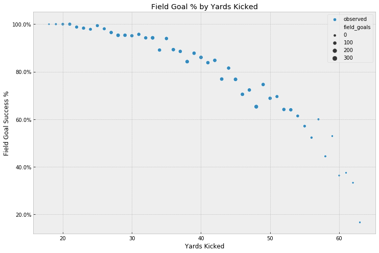
We notice that it gets pretty thin after 55 yards or so. Again, this makes intuitive sense - coaches wouldn’t risk a field goal attempt at anything less than a 50% chance and would probably just punt the ball to get it out of their side of the field.

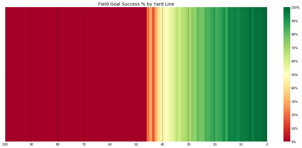
Mapping this onto a 100 Yard Football field, we see how this translates into field position:

What are we modeling?

For this post, we’re interested in the calculating the probability of making a field goal, given what we might know at the time the kicker gets called on to the field. This is similar to our problem setup when we modeled Fourth Down Attempts. The difference is that this time around, we don’t just want to model the latent probability, but we want to model it conditional on a number of external factors. For example, the distance of the kick we’re about to attempt is a key contributor to success or failure.

One obvious choice for modeling this problem is the data science classic logistic regression. In logistic regression, we want to model the probability of an event given a number of factors (or features/covariates) so that we can predict a binary outcome. (If we have more than two possible outcomes, we would use multinomial logistic regression, also sometimes referred to as softmax regression.)

Ford v Ferrari Bernoulli v Binomial

If you’ve used logistic regression in a machine learning context, you’ll have likely used the version implemented in the popular scikit-learn package⁵. In scikit-learn, we would have to set up our data so that the response variable is a binary outcome. Each row represents what is known as a Bernoulli trial, i.e. an individual outcome. So, in our case, each row would have to represent a single kick attempt, including the boolean is_field_goal_success as the response variable.

| play_id | kick_distance_yards | is_field_goal_success |
|---------|---------------------|-----------------------|
| 2278    | 19.0                | True                  |
| 1336    | 35.0                | True                  |
| 3290    | 54.0                | True                  |
| 3034    | 50.0                | True                  |
| 1121    | 46.0                | False                 |
| 3687    | 50.0                | True                  |
| 1964    | 51.0                | True                  |
| 2826    | 22.0                | True                  |
| 459     | 25.0                | True                  |
| 1351    | 47.0                | True                  |

In our xa_field_goals dataset we have over 13,500 field goals across 11 regular seasons. That’s a “small data” set and computationally likely not challenging in any model. However, depending on the features we want to model, we’d likely be better off with aggregate data.

For example, if our only feature is kick_distance_yards, we’d do well to aggregate all plays by kick distance and sum up the field_goals and successful_field_goals columns to arrive at a much smaller dataset, with less than 50 rows. These aggregate rows correspond to a Binomial representation of the data, which implies that there is a probability $p$ of an event happening, given $n$ attempts and given that we’ve observed $y$ successful events.

| kick_distance_yards | field_goals | successful_field_goals |
|---------------------|-------------|------------------------|
| 18.0                | 17          | 17                     |
| 19.0                | 123         | 123                    |
| 20.0                | 251         | 249                    |
| 21.0                | 300         | 294                    |
| 22.0                | 332         | 326                    |
| 23.0                | 368         | 362                    |
| 24.0                | 294         | 282                    |
| 25.0                | 358         | 354                    |
| 26.0                | 317         | 307                    |
| 27.0                | 369         | 354                    |

While the base implementation of logistic regression in R supports aggregate representation of binary data like this and the associated Binomial response variables natively, unfortunately not all implementations of logistic regression, such as scikit-learn, support it.

However, since we’ll be implementing this more explicitly in PyMC3 as a Bayesian model, we’ll get to choose our likelihood function. This is one of the big benefits of Bayesian modeling in a probabilistic programming framework. While there isn’t a neat built-in list of estimators, we can build our implementations in a plug-and-play fashion, using the built-in distributions as flexible building blocks.

So, if this represents a standard logistic regression model with a Bernoulli likelihood,

\[\begin{aligned} \alpha \sim Normal(0, 1) \\ \beta \sim Normal(0, 1) \\ z = \alpha + \beta * X_i \\ p_i = sigmoid(z) \\ y \sim Bernoulli(n, p_i) \\ \end{aligned}\]

we’ll change out the likelihood for a Binomial distribution for our model:

\[\begin{aligned} \alpha \sim Normal(0, 1) \\ \beta \sim Normal(0, 1) \\ z = \alpha + \beta * X_i \\ p_i = sigmoid(z) \\ y \sim Binom(n, p_i) \\ \end{aligned}\]

Here, $sigmoid$ represents the sigmoid or inverse logistic function that’s need to turn z into a probability:

\[p_i = \frac{1}{1 + e^{-z_i}}\]

In a prediction context, this $p_i$ would then be used to determine a binary outcome, where the $sigmoid$ function becomes an “activation” function, mapping probabilities to the output space (0/1).

\[\begin{split} p \geq 0.5, class=1 \\ p < 0.5, class=0 \end{split}\]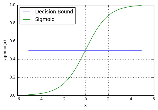

(credit: ML Cheat Sheet)

Note, however, that, as we saw earlier, given our class imbalance, this decision function would likely classify all our of our predicted probabilities as True, unless we took extra steps to deal with the imbalance. In our case, this is fine since we won’t use this to predict a binary outcome. Intuitively, this also makes sense. Coaches won’t call a field goal unless they’re fairly certain their kicker can make the play. So, their own prediction of field goal success for an attempt is always True.

Calibration

Since we’re mostly interested in the estimated field goal probabilities, a nice property of logistic regression is that the resulting probabilities are already calibrated, so they can be directly interpreted as a confidence level. So, if a logistic regression model predicts 90% probability for a certain class, 90% of the samples used in training it should actually belong to that class.⁶

(1) Baseline Model - Logistic Regression - Yards Kicked

For our baseline model, we’ll use the actual yards kicked, kick_distance_yards as our sole predictor.

In PyMC3, there are a number of ways to set this up - explicit parameters, matrix formulation or using the GLM module. For this model, we’ll look at how to set this up explicitly.

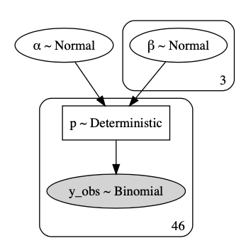
Assuming we have a pandas data-frame called df_train_yards that contains the total field goal attempts field_goals and successful field goals successful_field_goals by yards kicked kick_distance_yards, this model will recover the posterior probability of making a field goal by kick distance via its parameter p:

X = df_train_yards["kick_distance_yards"].values
n = df_train_yards["field_goals"].values
y = df_train_yards["successful_field_goals"].values

with pm.Model() as model_logit_yards:

    α = pm.Normal("α", mu=0, sd=1)
    β = pm.Normal("β", mu=0, sd=1)


    z = α + β * X
    p = pm.Deterministic("p", pm.math.invlogit(z))

    y_obs = pm.Binomial("y_obs", n=n, p=p, observed=y)

After sampling via MCMC (NUTS), we get the following coefficients:

|   | mean   | sd    | hpd_3% | hpd_97% |
|---|--------|-------|--------|---------|
| α | 6.035  | 0.188 | 5.687  | 6.387   |
| β | -0.106 | 0.004 | -0.113 | -0.098  |

(Your results may vary a bit even with the same random seed value, since this is stochastic.)

How do we interpret these coefficients?

In logistic regression, the coefficients represent the increase in log-odds for every unit increase in $X$. So, in our case for every additional yard a kicker has to kick, the log-odds of making the goal decrease by 0.106 over the baseline. We can turn these log-odds into probabilities by applying the $sigmoid$ function (a version of which we also applied in our PyMC3 model) to the regression model.

So, for example, a kick from 35 yards out has a probability of success of ~91%:

import numpy as np

def sigmoid(x):
    return 1 / (1 + np.exp(-x))

yards = 35
z = trace_logit_yards["α"] + trace_logit_yards["β"] * yards
sigmoid(z).mean()

0.9119025067736969

(Note that we’re taking the sigmoid function of the entire term, $\alpha + \beta * X$, and then we take the mean of all the samples in our trace.)

Plotting our model parameter $p$ against yards kicked, we get the following model results:

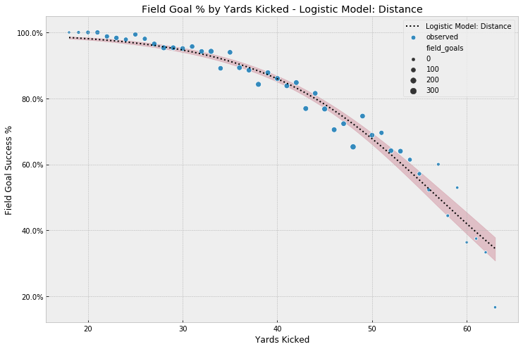
We see that our baseline model does a pretty good job modeling the observed data. However, it doesn’t do a good job modeling the attempts very close to the goal, and those a lot further out. For attempts close the goal line we have to remember that no field goal in our dataset has been attempted at anything less than 18 yards. (In that scenario, the line of scrimmage is at the 1 yard line.) So, remembering the way we calculated the probabilities of making the kick earlier, we see that given our model, the best we can do is ~98%,

yards = df_train_yards["kick_distance_yards"].min()
sigmoid(trace_1["α"]+ trace_1["β"] * yards).mean()

0.984129147435348

If there was such a thing as a kick from 0 yards, we still have the intercept $\alpha$, which would leave us with a probability of close to 1.0 (sigmoid(trace_1["α"]).mean() = 0.9975696388564776).

(2) Kick Geometry Model

Another way to think about modeling field goals, is to approach it from a first-principles approach taking the geometry of a field goal kick into account. Andrew Gelman demonstrates a similar approach in his Stan case study on golf putts⁷. Andrew went into great detail on the angles and physical forces involved in putting and showed how, if expressed mathematically, they can be modeled probabilistically - in that case with great success.

I’m not an expert on the physics of ball kicks, and I haven’t had geometry since before I started shaving, but the point of this section is to show how flexible the Bayesian modeling approach is. If we have a reasonable mental model of how our data was generated, we can use the building blocks of our probabilistic programming framework of choice (here PyMC3) to build the “machine” that might have generated it and evaluate this model based on its fit.

Colin Carroll did a great job porting Andrew Gelman’s case study to PyMC3 and we will lean heavily on his work for this post.⁸

Breaking down a kick into some basic components, we can reason that we have to consider:

• the chance that the kicker misses the goal posts horizontally, i.e. he kicks too far left or right
• the chance that the kick comes up short

The probability $p$ of making the goal is the joint probability of:

P(Kick is within the required angle) * P(Kick is not short)

This is somewhat analogous to Andrew’s geometry-based model of golf putts, with the exception that unlike in golf, we don’t care if the field goal is too long.

So, given some properties of the field goal posts, we assume that:

• the goal is 18.5 feet wide
• kicks are initiated from the right or left hashmark, which is 10.75 feet from the edge of the goal post

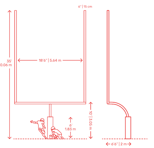
(Credit: https://www.dimensions.guide/element/field-goal-post)

Horizontal Angle

Armed with this information, we can think of the angle of a field goal as the angle \(\beta\) - \(\alpha\) in this diagram (from this post by David Park)

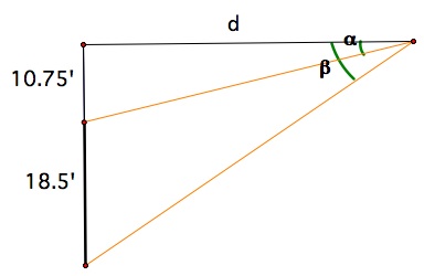
It gets a little fuzzy when you’re trying to determine from which spot a kicker might have actually kicked the ball, since there seems to be some discretion on whether to kick from the center line, or from one of the hashmarks⁹. For this model, let’s assume the kicker kicks from one of the hashmarks.

From this, we can calculate this angle based on the distance to kick as:

\[\beta = ArcTan(\frac{29.25}{distance})\] \[\alpha = ArcTan(\frac{10.74}{distance})\] \[angle = \beta - \alpha\]

Or in Python:

DISTANCE_TO_HASHMARK_FT = 10.75
GOAL_WIDTH_FT = 18.5

def get_kick_angle_horiz(distance_yards):
    adjacent_ft = distance_yards * 3
    opposite_ft_total = DISTANCE_TO_HASHMARK_FT + GOAL_WIDTH_FT
    opposite_ft_side = DISTANCE_TO_HASHMARK_FT

    β = np.arctan(opposite_ft_total/adjacent_ft)
    α = np.arctan(opposite_ft_side/adjacent_ft)
    return β - α

Note that this function returns the angle in radians, which is computationally convenient but not all that intuitive for most people, so we’ll convert it to degrees for plotting and reporting:

def radiants_to_degrees(y):
    return (y*180.0/np.pi)

Let’s take a look at how this angle changes with distance:

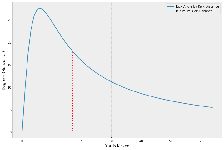
So, with the understanding that in reality kick distances start at 18 yards (historically), we see that the required angle gets smaller and smaller as we get away from the goal. It also decreases in a non-linear fashion, which tells us that there is some useful information in the angle calculation we couldn’t just get from distance alone.

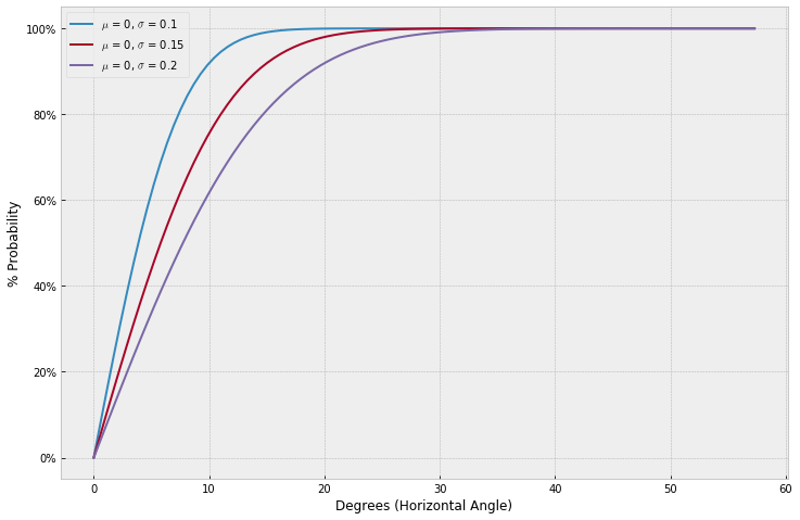
Following Andrew Gelman’s post on putts, we can adapt his calculation of the probability of kicking the ball within that angle, using a cumulative normal distribution:

\[\beta = ArcTan(\frac{29.25}{distance})\] \[\alpha = ArcTan(\frac{10.74}{distance})\] \[\mbox{Pr}\left(|\mbox{angle}| < (ArcTan(\frac{29.25}{distance}) - ArcTan(\frac{10.74}{distance}))\right)\] \[= 2\Phi\left(\frac{ArcTan(\frac{29.25}{distance}) - ArcTan(\frac{10.74}{distance})}{\sigma_{\rm angle}}\right) - 1\]

Being less mathematically literate, I like to visualize these things to make this more clear. If we plot this model for a few different values of \(\sigma_{\rm angle}\), we see why a cumulative distribution makes sense here. The bigger the angle gets (i.e. the closer we are to the goal line), the more likely it is we kick the ball within that angle. Or conversely, the farther away we have to kick, the harder it gets to get within the required angle. We also note that, depending on kick accuracy within the angle, at a certain angle, it no longer poses a hurdle in kicking and we see the probability of kicking at the required angle asymptote at 100%.

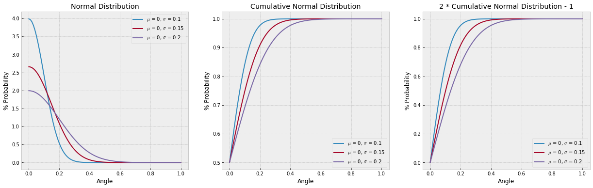
It might also help to look at how Andrew Gelman derives the formula for expressing the cumulative probabilities by angle. Since we’re only dealing with positive values on the x-axis, we need to multiply by 2 and subtract 1 to bring this back to unit scale:

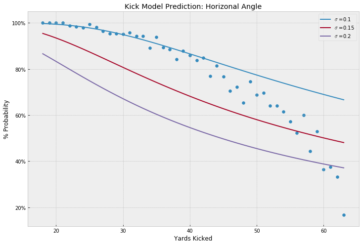
The kickers’ latent variance in making the goal in this model, \(\sigma_{\rm angle}\) , is unknown for the population of kickers, so we will want to estimate it from our data.

Overlaying the modeled probabilities for a few values for kicker variance by yard kicked with the actuals, we see the angle alone is likely not a great model for field goal %:

Force of Kick

We can characterize the second component of our geometry-based model as the force of the kick, or the probability that the kick will be kicked hard enough to make the distance to the goal, plus a foot. Unlike Andrew’s golf putt model, we’re not concerned with overshooting the goal, and only concerned about coming up short.

So, again borrowing from Andrew’s work, we could formulate the probability of making it over the goal by 1 foot as:

\[\Phi\left(\frac{1}{(distance+1)\,\sigma_{\rm distance}}\right)\]

Overlaying the modeled probabilities for a few values for kicker variance by yard kicked with the actuals, we see our distance model alone may be good up to about 35 feet but does a poor job accounting for the probabilities further out:

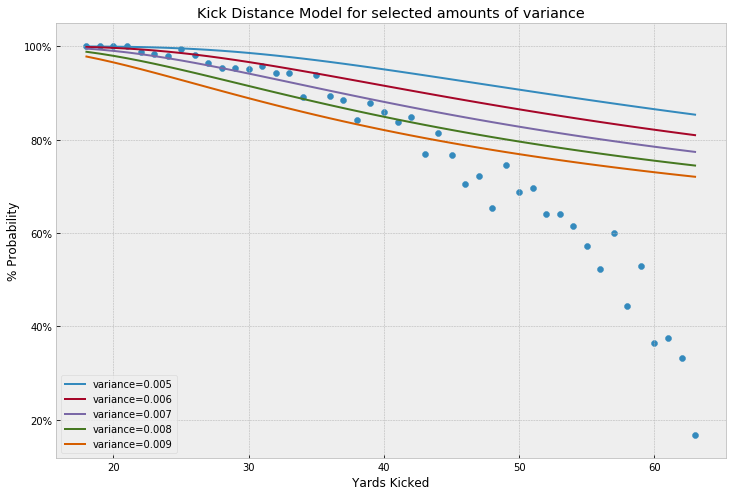
Combining both models’ joint probabilities, plotted with a number of selected variance combinations, gives us more comprehensive view of what this model could cover. However, we notice that the model, in any of the plotted combos, fails to account for the drop-off in kick success probability as kicking yards increase:

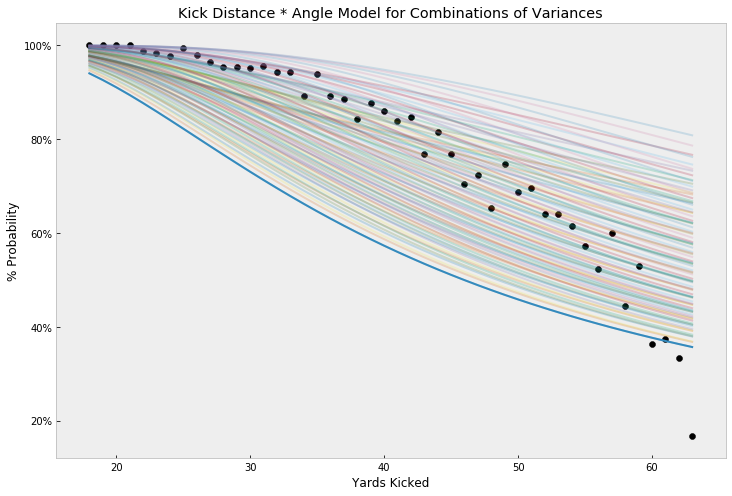
Clearly, there are other physical factors to explore in future work, but for the time being, let’s leave it here and estimate this model’s latent parameters’ posterior distribution to get a sense of uncertainty in the model.

Using a theano implementation of $\phi$,

import theano.tensor as tt

def Phi_tt(x):
    return 0.5 + 0.5 * tt.erf(x / tt.sqrt(2.))

we can express the model we set up above in PyMC3 like so:

with pm.Model() as model_geo:

    σ_angle = pm.HalfNormal("σ_angle", sd=1)
    σ_distance = pm.HalfNormal("σ_distance", sd=1)

    over_ft = 1
    X_distance_ft = X_distance*3

    p_angle = pm.Deterministic("p_angle", (2 * Phi_tt(X_kick_angle_horizontal / σ_angle) - 1))

    u = (over_ft) / ((X_distance_ft + over_ft) * σ_distance)
    p_distance = pm.Deterministic("p_distance", Phi_tt(u))

    p = pm.Deterministic("p", p_angle * p_distance)

    y_obs = pm.Binomial("y_obs", n=n, p=p, observed=y)

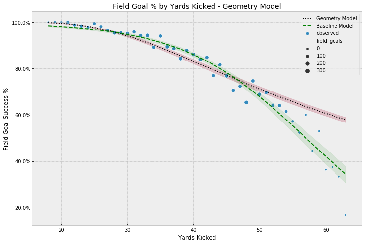
After sampling, we compare our posterior, including uncertainty estimates (via a 95% HPD), to the observed values. Compared to our baseline model, the geometry-based model does a better job modeling the probabilities for shorter kicks, but as we saw in our setup, fails to adequately account for the intricacies of longer kicks.

(3) Logistic Regression - Yards Kicked & Angle

Seeing that our baseline model, logistic regression on yards kicked, provides a fairly good fit and having learned some about the geometry of field goal kicking, it may make sense to return to logistic regression and add the horizontal angle of the kick to the model as a predictor. Since we now have two predictors, we can use this as an opportunity to look at a matrix approach in formulating regression models in PyMC3.

We’ve precomputed the angle in a our nfl-dbt model in degrees to bring the units into the same order of magnitude as kick yards without having to standardize the variables (the regression police would probably take offense to this), and we can now include it as a feature in the design matrix $X$:

feature_columns = ["kick_distance_yards", "kick_angle_horizontal_degrees"]

X = df_train_yards[feature_columns]

We now want to model two values for $\beta$, so we make use of the shape parameter to have PyMC3 create as many slope coefficients as we have columns in $X$. We then compute $z$ as the $dot$ product of $X$ and $\beta$ before again converting $z$ to probabilities via the invlogit function:

with pm.Model() as model_logit_yards_angle:

    α = pm.Normal("α", mu=0, sd=.1)
    β = pm.Normal("β", mu=0, sd=.1, shape=X.shape[1])

    z = α + pm.math.dot(X, β)

    p = pm.Deterministic("p", pm.math.invlogit(z))

    y_obs = pm.Binomial("y_obs", n=n, p=p, observed=y)

The resulting parameter estimates show that we have a negative effect as distance increases and a positive effect as the angle increases.

|      | mean   | sd    | hpd_3% | hpd_97% |
|------|--------|-------|--------|---------|
| α    | 0.024  | 0.099 | -0.159 | 0.212   |
| β[0] | -0.037 | 0.002 | -0.041 | -0.032  |
| β[1] | 0.366  | 0.013 | 0.342  | 0.391   |

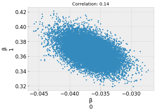
You’d think that these two parameter would be highly collinear, presenting sampling problems, but looking at the correlation between posterior samples for $\beta_0$ and $\beta_1$ shows very little correlation:

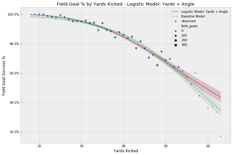
Comparing this model’s output to our baseline model, we see that the addition of the angle improved the fit for very short kicks and perhaps made the model more robust to small data outliers from kicks past 55 yards:

(4) Logistic Regression - Yards Kicked & Angle + Interactions

For our final model expansion, it seems reasonable to assume that both distance and angle play a combined factor in a kicker’s success. So, in addition to the independent covariates, let’s also model the interaction term between the two.

Continuing our matrix-based setup from the prior model, we just need to add the interaction to our design matrix $X$,

df_train_yards["kick_distance_yards_angle"] = (
    df_train_yards["kick_distance_yards"] *
    df_train_yards["kick_angle_horizontal_degrees"]
)

feature_columns = ["kick_distance_yards", "kick_angle_horizontal_degrees", "kick_distance_yards_angle"]
X = df_train_yards[feature_columns]

The rest of the model stays the same, but we get an additional $\beta$ parameter:

After sampling, we can see that our interaction term coefficient $\beta_2$, while greater than $0$, is small with a wide uncertainty interval. From an interpretability standpoint, it’s also hard to reason about an effect of yards*angle, so this additional parameter falls more in the category of feature extraction to improve model fit.

|      | mean   | sd    | hpd_3% | hpd_97% |
|------|--------|-------|--------|---------|
| α    | 0.003  | 0.102 | -0.193 | 0.189   |
| β[0] | -0.067 | 0.013 | -0.092 | -0.043  |
| β[1] | 0.237  | 0.056 | 0.131  | 0.343   |
| β[2] | 0.007  | 0.003 | 0.001  | 0.012   |

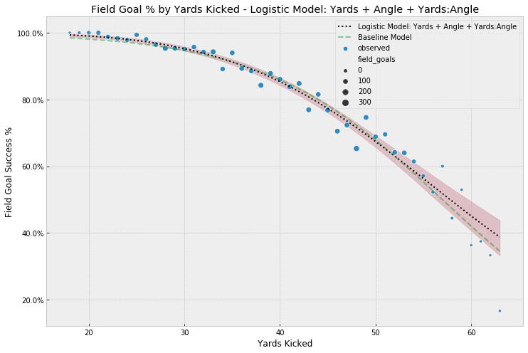
Interestingly, this last model provides the widest uncertainty interval for longer kicks yet, likely best reflecting the lack of data and clear factors contributing to success from those distances.

Model Comparison & Evaluation

As I mentioned in part 1 of this series, as part of our workflow we should also formally compare the 4 models. Using leave-one-out cross-validation¹⁰, we see that the last two models, logistic regression including kick angle and the model including the interaction term, score best (lowest values for deviance):

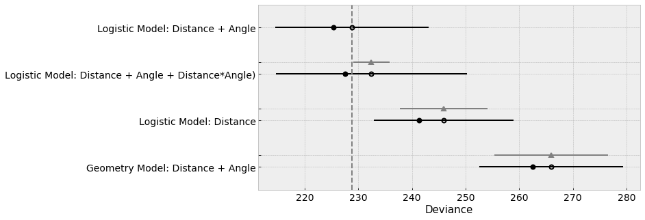
The model including the interaction term likely gets a slightly worse score here because of its wider uncertainty interval.

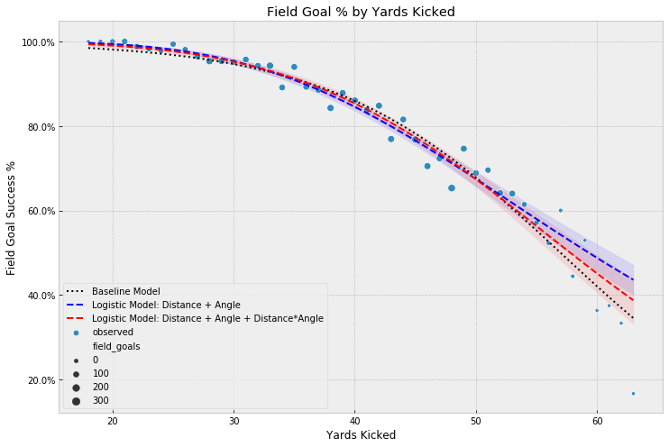
However, comparing those two models plotted against yards kicked, we may want to favor the model with the interaction term for its better fit on longer kick probabilities, while maintaining comparable fit across the other kick distances:

Summary

Hopefully this post highlighted some of the benefits of Bayesian modeling using a probabilistic framework, in particular the flexibility in constructing models and the ability to estimate usable uncertainty intervals. I’ll be highlighting other aspects of Bayesian modeling, such as multi-level modeling in future posts, so stay tuned!

Notes

1. Wikipedia: Field goal ↩

2. Why You Should Watch the Field Goal Kicker When Betting on Football ↩

3. NFL Salary Rankings ↩

4. Justin Tucker Believes He Can Hit An 84-Yard Field Goal ↩

5. scikit-learn docs - Logistic Regression ↩

6. scikit-learn docs - Probability Calibration ↩

7. Model building and expansion for golf putting, Andrew Gelman ↩

8. There is also a port of the golf putt model to Julia’s Turing package by Josh Duncan Model building of golf putting with Turing.jl ↩

9. What is field goal range? How is field goal distance measured? ↩

10. Practical Bayesian model evaluation using leave-one-out cross-validation and WAIC ↩