Bayesian Modeling of NFL Football Fourth Down Attempts with PyMC3

In this post, we’ll model a key NFL football statistic, Fourth Down Attempts using Bayesian Modeling and PyMC3. Hopefully, this will part of a series of posts (and accompanying Jupyter notebooks) on exploring NFL stats using a variety of analytics techniques in the coming months.

Motivation

I’ve been looking for a good data science teaching dataset for a while, one that can be used for regression, classification, forecasting and other analytical modeling. The NFL Play-by-Play dataset we’ll get to know in more detail below is a great candidate.

Hopefully, time permitting, over the next few months we’ll explore it from a few different angles:

• Loading and transforming raw data in BigQuery with dbt
• Modeling specific stats, such as fourth down attempts or NFL Passer Ratings in a Bayesian framework (today’s is one of those posts)
• Predicting play outcomes, such as pass completions using non-linear models, such as Random Forest/GMBs/xgboost
• Modeling drives down field with survival models

Please note that this isn’t a football or a sports analytics blog. While I attempt to bring as much domain knowledge into any analysis, the point of these posts is to present analytical concepts, not to compete with ESPN.com. Having said that, I’d love your feedback on how to improve this analysis if you know your way around football stats.

What are Fourth Down Attempts and Conversions?

Feel free this skip this if you know all about the sportsballs

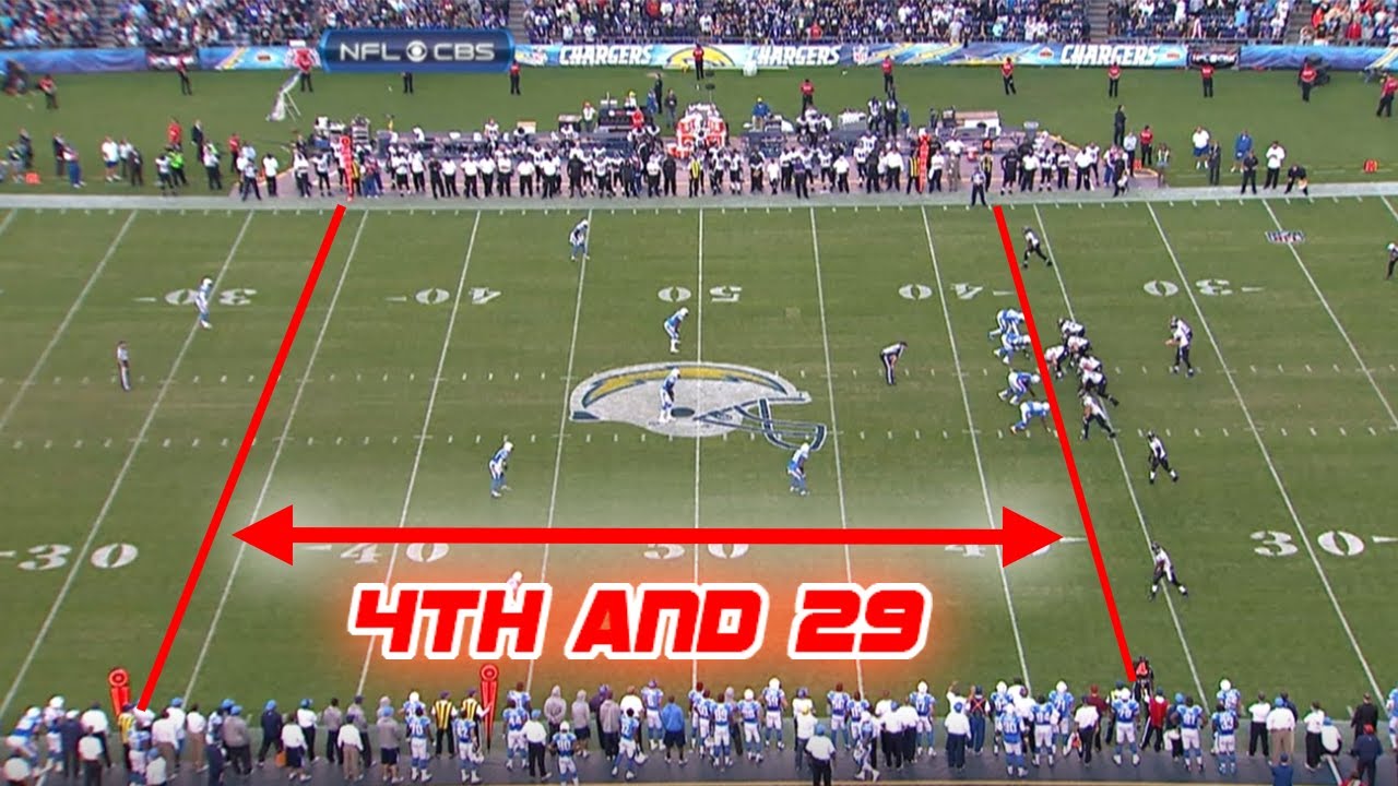
In American Football, in broad strokes, a team gets 4 tries, known as “downs”, at gaining at least 10 yards cumulatively during a drive. When a team gains the required 10 yards, the count resets and they’ll try again until the team either reaches the end zone for a touchdown (or is close enough to at least kick a field goal), or fails at gaining the required ground and the ball is turned over to the opposing team, or the clock runs out.

Much is made about a team’s ability to convert on the crucial third down, which is usually seen as the last down to try for either a run or a pass. The fourth, or last possible down is often seen as too risky to go for a pass or a run, as failure to do so would result in a turnover on the spot. Consequently, many coaches opt to punt, i.e. kick the ball, on fourth down to move the opposing team’s starting position downfield. And so, one of the most popular sports metaphors was born.

However, there has been much discussion about whether NFL teams are “going for it”, as the idiom goes, often enough¹. In fact, the New York Times in 2013 even created a 4th Down Bot² to model the expected value of fourth down attempts by field position, which concluded that most coaches are in fact not aggressive enough on fourth down and, thus, give up their chance at scoring on a drive.

Getting NFL Play-by-Play Data

To start, I sourced play-by-play data for the 2009 through 2019 regular seasons from the very helpful nflscrapR-data repository on Github³.

This repo also include pre and post-season data, along with team rosters - data I’ll hope to explore in future posts.

[In fact, the data in this repo is generated via the NFLScraperR library for R⁴ and seems to be updated weekly.]

To make the csv files easier to work with, I loaded the data into a BigQuery dataset and unioned all seasons together after cleaning up a few things. For this particular post, we’ll use only a subset of columns, and only plays on fourth down that did not result in a field goal.

| play_id                  | 2602       | 3224       | 3359       | 3611       | 3705       | 3802       | 4086       | 4173       |
|--------------------------|------------|------------|------------|------------|------------|------------|------------|------------|
| season_code              | R2019      | R2019      | R2019      | R2019      | R2019      | R2019      | R2019      | R2019      |
| game_id                  | 2019111800 | 2019111800 | 2019111800 | 2019111800 | 2019111800 | 2019111800 | 2019111800 | 2019111800 |
| quarter                  | 3          | 4          | 4          | 4          | 4          | 4          | 4          | 4          |
| drive                    | 13         | 16         | 17         | 18         | 19         | 20         | 22         | 23         |
| play_time                | 8:32:00    | 14:50:00   | 12:26:00   | 8:12:00    | 6:18:00    | 4:40:00    | 2:00:00    | 1:25:00    |
| off_team_code            | LAC/SD     | KC         | LAC/SD     | KC         | LAC/SD     | KC         | KC         | LAC/SD     |
| off_team_type            | home       | away       | home       | away       | home       | away       | away       | home       |
| def_team_code            | KC         | LAC/SD     | KC         | LAC/SD     | KC         | LAC/SD     | LAC/SD     | KC         |
| play_type                | no_play    | punt       | punt       | punt       | punt       | punt       | punt       | pass       |
| is_field_goal_attempt    | False      | False      | False      | False      | False      | False      | False      | False      |
| is_fourth_down_attempt   | False      | False      | False      | False      | False      | False      | False      | True       |
| is_fourth_down_converted | False      | False      | False      | False      | False      | False      | False      | True       |

[Sample of rows, transposed]

The data for this post, along with a more detailed Jupyter notebook containing all the code for the post are in the Github repo accompanying this series, https://github.com/clausherther/nfl-analysis

For this post, let’s consider fourth down tries to be plays on fourth down that did not result in a field goal attempt. The reasoning here is that as we attempt to model teams’ propensities to go for it on fourth down, we shouldn’t penalize them for not going for a pass or run, if they were close enough for a field goal.

Conforming Team Names

Over the years, NFL teams such as the L.A. Rams and Chargers have moved cities, and thus changed team names. For the purposes of this analysis, we’ve conformed names for teams that have moved. So, the L.A. Rams, having moved back from St. Louis are known as LA/STL in our dataset. Similarly, the L.A. Chargers, having moved from San Diego, are shown as LAC/SD.

Training Period - Mid Season

As I’m writing this, we’re in week 13 out of 17 for the regular 2019 NFL season, and our data set has games through November 25th, 2019. With 2/3 of the regular season behind us, it’d be interesting to see how certain we can be about our analysis of 2019 vs prior years.

Visual Data Exploration of Fourth Down Attempts

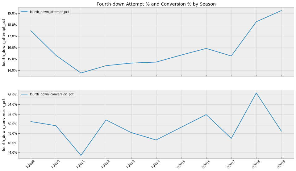
From the plots by season below we can see that there might be a recent uptrend in attempt %, and while there could be a longer term upwards trend in conversion % the uptick in 2018 is so far not continuing in 2019.

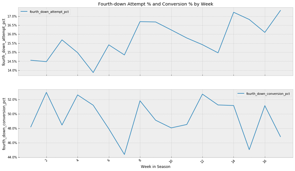
Interestingly, looking at this by week in the season, teams seem to be getting more aggressive going for it on fourth down as the season goes on, but they don’t appear to get any better at converting those attempts throughout the season.

Looking at a heatmap of fourth down attempt % by teams vs seasons, we can possibly spot a couple of trends that we’ll be confirming. For example, we see slightly higher numbers in the last 2 seasons (driven by a few teams such as BAL and ‘NYG). Also, you’ll notice that the Philadelphia Eagles (PHI) have had consistently higher fourth down attempt percentages the last few seasons.

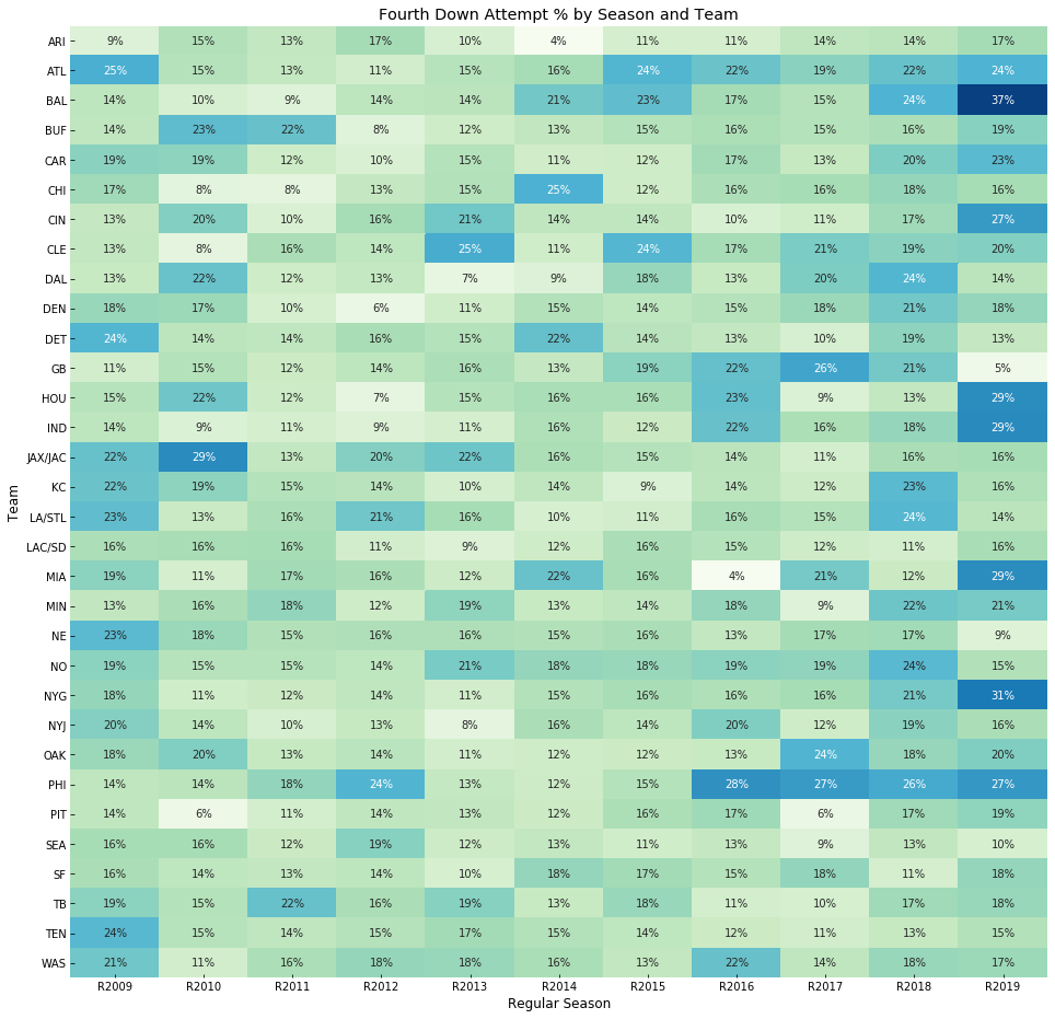
So, a few takeaways from our data exploration that are worth analyzing further:

• Attempt % by season seems to be increasing
• Teams seem to get more aggressive on fourth down as week in the season go by
• Some teams, notably PHI seem to be more aggressive than others on fourth down in recent years

Fourth Down Attempts, Bayesian Style

What is Bayesian Workflow?

For our analysis, we’re going to model fourth down attempts and conversions using a Bayesian model:

A Bayesian model is a statistical model where you use probability to represent all uncertainty within the model, both the uncertainty regarding the output but also the uncertainty regarding the input (aka parameters) to the model. ⁵

One advantage to a Bayesian model is that it allows us to draw inferences about our data with many fewer data points than a traditional machine learning model would require. If we wanted to model the percentage of fourth down attempts by football season, using summarized season-level data - i.e. in our case 11 data points - would be sufficient to build a usable model. This has important real-world applications, as so many of the more interesting areas of data science are in the small-to-medium data world.

[If you’re interested in learning more about Bayesian modeling, Richard McElreath’s book “Statistical Rethinking”⁶ is a great introduction (and beyond) to the topic.]

Moreover, in contrast to many Machine Learning approaches, Bayesian modeling requires us to think harder about the subject we’re trying to model in order to understand the nuances and possible pitfalls of our choices better.

Andrew Gelman demonstrates this beautifully in his case study on using Stan to model golf putts, “Model building and expansion for golf putting”⁷, in which he ultimately employs insights from a knowledgeable golfer to build a model from first principles.

I won’t go quite as far in this post, mostly for lack of professional football player friends, but I’ll follow Andrew’s workflow in broad strokes:

1. Model building: in this step we’ll build a mathematical model based on what we know about the subject. Here we’ll also define, and in the process question our choice of prior distributions for the random variables we’re modeling. During this step, practitioners often also use synthetic data to build their model before introducing observed data to the model which helps verify that the hypothesized generative process works with the model and priors we’ve chosen. Similarly, checking prior predictive distributions (data generated from our priors) can be very helpful here, particularly for more complex models.

2. Inference: we’ll use PyMC3 and MCMC, specifically the NUTS variant of the Hamiltonian Monte Carlo sampler because of its efficiency and sampling the posterior space

3. Model Critique: in this crucial step, we’ll make sure our sampler converged and check our posterior distributions for fit and reasonability, checking a few convergence statistics, such as $\hat{R}$ and effective sample sizes⁸. Since we’ll be building multiple models, we’ll employ quantitative approaches to gauge our models’ fit, using techniques such as WAIC and leave-one-out cross-validation⁹.

4. Model Expansion: lastly, we’ll repeat the process if needed, adding additional variables or levels to our model to better capture the data generating process.

[Schad, Betancourt and Vasishth proposed a more formal set of steps in their paper “Principled Bayesian Workflow”¹⁰ if you’re interested in diving deeper here.]

Model Data

For all our models, we’ll use summarized fourth down play data. Instead of the individual 32,628 fourth down plays in our play-by-play dataset, we will make our life (and our MCMC sampler’s life) easier by aggregating those plays by:

• Season
• Week
• Team

With this combination, we’ll be able to satisfy our modeling requirements for this post.

For the 11 seasons, at 32 teams with ~16 games each (~10 for 2019), we end up with ~5,400 data points - manageable in size, but rich in information.

Baseline Model

Let’s consider our first question for our dataset: are NFL teams getting more aggressive in “going for it” on fourth down? To try to answer this question, let’s think of the generative process for fourth down attempts, denoted by $y$. In simple terms, it’s a factor of the number of fourth downs a team has over a season, let’s use $X$, and a latent, i.e. unknown, propensity to “go for it”, $\theta$

\[y = \theta * X\]

This setup is strikingly similar to a classic coin flip example, where the coin has an unknown bias that we’d like to to estimate. You could easily imagine a coach flipping his lucky coin every time the team faces a fourth down to determine whether to punt or to go for it.

Canonically, coin flip outcomes can be modeled using a Binomial distribution, and the process of flipping a coin is often modeling using a Beta-Binomial model. In such a model, a Beta distribution is used to model the coin’s bias (i.e. the latent proportion of heads vs tails) and a Binomial distribution is used to model the outcomes of n coin flips given this latent bias.

\[\alpha \sim HalfNormal\] \[\beta \sim HalfNormal\] \[\theta \sim Beta(\alpha, \beta)\] \[y \sim Binomial(n, \theta)\]

I’ve written previously about Beta-Binomial models and their extension, Dirichlet-Multinomials in Dice, Polls & Dirichlet Multinomials.

Model Building

As a baseline model, let’s set up a simple Beta-Binomial model to gauge the latent bias towards “going for it” across all seasons, weeks and teams. This is also known as a pooled or fully-pooled model, since we’re combining information across all of our groups. Chris Fonnesbeck wrote a great post, “A Primer on Bayesian Methods for Multilevel Modeling”¹¹, for the PyMC3 docs that I recommend reading for more on this.

with pm.Model() as attempts_base_line_model:

    alpha = pm.HalfNormal("alpha", sd=1)
    beta = pm.HalfNormal("beta", sd=1)

    theta = pm.Beta("theta", alpha=alpha, beta=beta)

    y = pm.Binomial("y", n=X_obs, p=theta, observed=y_obs)

As you can see, PyMC3 gives us a straightforward way to express the mathematical notation above in Python.

We can also show our model graphically in plate notation:

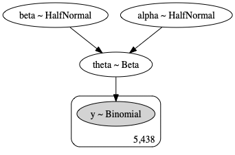
A quick overview of this model:

• The number of fourth down attempts y_obs are modeled with a $Binomial$ likelihood
• The number of fourth down tries are provided as an input, X_obs
• The latent bias/probability of “going for it” on fourth down, theta is modeled with a $Beta$ prior, reflecting our knowledge that proportions cannot exceed 100%. Thus, the $Beta$ distribution, bounded by 0 and 1 makes a great candidate as a prior for proportions like this. This really is our parameter of interest, the posterior distribution of which we’d like to recover through our model.
• This $Beta$ prior is parameterized with two hyper-priors, alpha and beta, both modeled using $HalfNormal$ distributions (reflecting the fact that these parameters cannot be negative)

Inference

I’ll skip the code parts of running inference via MCMC for this post since PyMC3 makes that, thankfully, mostly trivial, but you’ll find it along with the necessary convergence checks in the accompanying notebook.

Model Critique

After sampling via MCMC/Nuts, we can now take a look at the posteriors of our variables, particularly $theta$.

PyMC3 includes a handy summary function that provides us with a few key estimates per variable. Aside from mean and the range covered in the hpd columns, we also want to make sure r_hat is ~1, while the effective sample sizes (ess) per variable are high enough to explore the posterior tails.

|          | mean  | sd    | hpd_3% | hpd_97% | mcse_mean | mcse_sd | ess_mean | ess_sd | ess_bulk | ess_tail | r_hat |
|----------|-------|-------|--------|---------|-----------|---------|----------|--------|----------|----------|-------|
| alpha    | 0.701 | 0.452 | 0.015  | 1.505   | 0.005     | 0.003   | 9253.0   | 9253.0 | 6777.0   | 4781.0   | 1.0   |
| beta     | 1.079 | 0.623 | 0.036  | 2.175   | 0.008     | 0.005   | 6646.0   | 6646.0 | 5055.0   | 3824.0   | 1.0   |
| theta    | 0.157 | 0.002 | 0.153  | 0.161   | 0.000     | 0.000   | 9099.0   | 9099.0 | 9113.0   | 7178.0   | 1.0   |

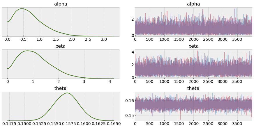
The arviz.plot_trace function gives us a quick overview of sampler performance by variable. We’re looking for efficient exploration of the posterior space, as shown in the plot below:

Plotting the posterior for theta from our baseline against a reference value (the mean of the observed data), we see that our baseline model estimates that between 15.3% and 16.1% of fourth downs result in a fourth down attempt. This is estimated across all seasons, teams and weeks.

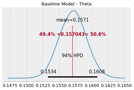
This indicates that our baseline model doesn’t really cover the variability of this metric from season to season and team to team very well. 2018’s average of > 18% for fourth down attempt % isn’t even in the 94% HPD (Highest Posterior Density) Interval. Similarly, the Philadelphia Eagles’ (PHI) fourth down attempt % of 26% in 2018 would be far out in the tails of this distribution and an outlier in this model.

Thus, while this baseline model converges and samples well, it only models the “average” combination of season, team and week and fails to model the nuances and heterogeneity of our dataset adequately.

Season Model

Model Building/Expansion

For our next model, an expansion of our baseline model, we’ll use the same data, but we’ll estimate Fourth Down Attempt % by Season, which we’ll model in a hierarchical model. Thus, we will estimate individual posteriors for each season, while also (partially) pooling data across all seasons.

This ability to partially pool data is one of the strengths of Bayesian modeling and allows us to draw strong inferences from small datasets.

The PyMC3 docs have some good insights here, particularly in the application to a similar sports-related problem set, baseball batting averages¹².

We will assume that there exists a hidden factor (phi) related to the expected performance for all players (not limited to our 18). Since the population mean is an unknown value between 0 and 1, it must be bounded from below and above. Also, we assume that nothing is known about global average. Hence, a natural choice for a prior distribution is the uniform distribution.

Next, we introduce a hyperparameter kappa to account for the variance in the population batting averages, for which we will use a bounded Pareto distribution. This will ensure that the estimated value falls within reasonable bounds. These hyperparameters will be, in turn, used to parameterize a beta distribution, which is ideal for modeling quantities on the unit interval. The beta distribution is typically parameterized via a scale and shape parameter, it may also be parametrized in terms of its mean μ∈[0,1] and sample size (a proxy for variance) ν=α+β(ν>0)

The final step is to specify a sampling distribution for the data (hit or miss) for every player, using a Binomial distribution. This is where the data are brought to bear on the model.

We could use pm.Pareto(‘kappa’, m=1.5), to define our prior on kappa, but the Pareto distribution has very long tails. Exploring these properly is difficult for the sampler, so we use an equivalent but faster parametrization using the exponential distribution. We use the fact that the log of a Pareto distributed random variable follows an exponential distribution.

So, following this example, which supplies us with a good amount of sports-analysis domain knowledge, we’ll also model $phi$ and $kappa$ hyper-priors to partially pool across seasons, and estimate season level $theta$ parameters.

Instead of a Binomial likelihood, we’ll use a Poisson likelihood, to account for the higher dispersion in fourth down attempts across seasons, teams and weeks.

Thus, we end up with a formulation like this, for each of our models for seasons, teams and weeks.

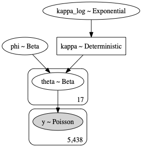
\[\begin{array}{l} \text{phi} \sim Beta(alpha, beta) \\\ \text{kappa_log} \sim Exponential(lam=3.0) \\\ \text{kappa} \sim exp(\text{kappa_log}) \\\ \text{theta} \sim Beta(\alpha=f(\text{phi},~\text{kappa}), \beta=f(\text{phi},~\text{kappa})) \\\ \text{mu} = X * \text{theta} \\\ y \sim Poisson(\text{mu}) \end{array}\]

Or, expressed in PyMC3:

with pm.Model() as attempts_season_model:
    
    # We use a Beta distribution here, 
    # parameterized to be uniform from 0 to 1
    phi = pm.Beta("phi", alpha=1, beta=1)

    # The rate parameter "lam" lets us control the amount
    # of regularization via our prior, where lower values
    # of "lam" provide stronger regularization 
    # ('rate' here being the inverse of scale)
    kappa_log = pm.Exponential("kappa_log", lam=3)
    kappa = pm.Deterministic("kappa", tt.exp(kappa_log))

    theta = pm.Beta("theta", 
                alpha=phi*kappa, 
                beta=(1.0-phi)*kappa, 
                shape=n_seasons)

    mu = X_obs * theta[season_idx]

    y = pm.Poisson("y", mu=mu, observed=y_obs)
    

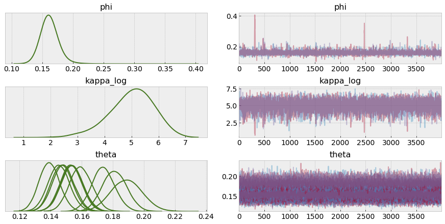
Let’s look at this in plate notation to make sure our levels are set up correctly:

Inference

After sampling using MCMC/Nuts, we again check our trace for any signs of misbehaved chains, and spot no issues or divergences:

Model Critique

Let’s take a look at the posterior for phi, which we’ve defined earlier as the parameter that estimates the probability of going for it on fourth down for the “population”, i.e. all seasons.

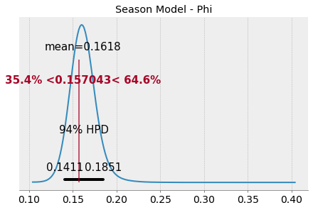
We’ll notice that the mean of the posterior for phi is slightly higher than our observed mean, and the distribution is long-tailed, capturing the fact that each season may have a much higher value than the average.

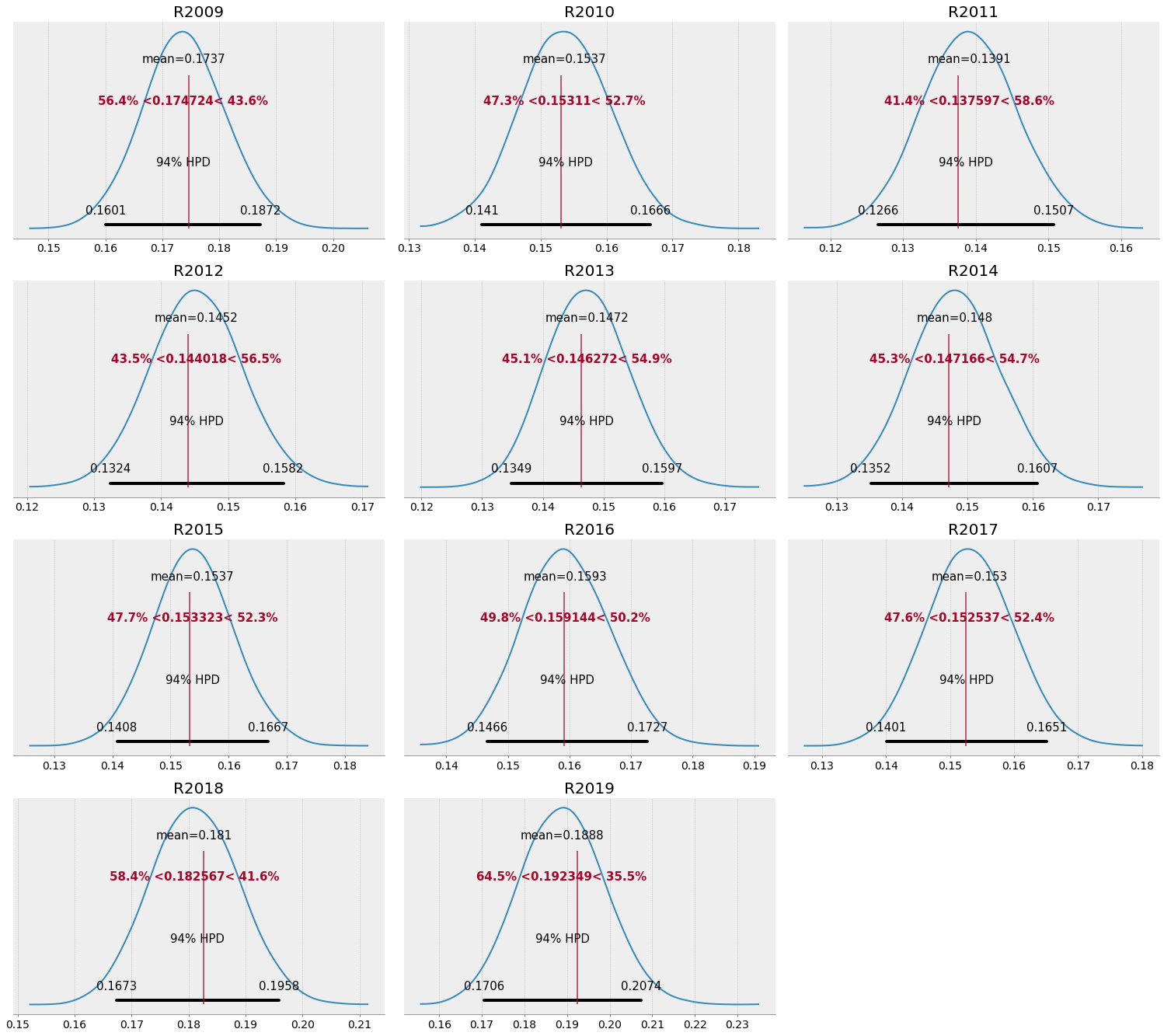
Plotting the posteriors for theta for each season, we can see how this model nicely captures the range for each season:

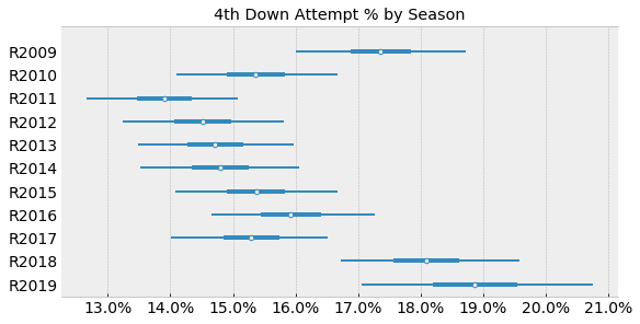
We see that 2018 and 2019 are clearly separated from the prior seasons. However, mid-season it’s still maybe too early to tell whether 2019 will indeed break a record for fourth down attempt % in the regular season.

Interestingly, even with stronger regularization via our priors, we don’t observe a lot of shrinkage of estimates towards the mean (an effect/benefit of partial pooling) for those season further away from the group. This is likely a result of strong evidence at the season level overwhelming our priors.

However, we can see some evidence of shrinkage visually by plotting our observed season values over the posterior distributions for theta by season. We notice that the posterior means for theta for both 2018 and 2019 are slightly lower than the observed values, while the low observed value for 2011 is below its posterior estimate - this is likely an effect of our model pooling information across seasons and adjusting estimates for those seasons accordingly.

Team Model

Moving on this our second model expansion. This time, we’ll follow the same approach we used for seasons, but pool our data by team. So, instead of 11 priors for theta, we have 32, thus allowing us to estimate posteriors for each team, based on all 11 seasons of weekly team level summary data.

We’ll skip the sampling and traceplot for the post (you can find that in the notebook) and go straight to looking at posteriors.

Model Critique

In this model, phi represents the population mean across teams, and we see that there is a lot less variability across teams on fourth down attempts than we saw in the baseline or season models:

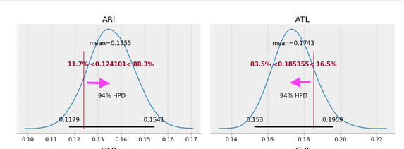
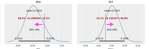
The forestplot of theta by team shows that aside from a few teams, most notably the Arizona Cardinals (ARI) and the Philadelphia Eagles (PHI), most teams hover around the ~15.7% group mean:

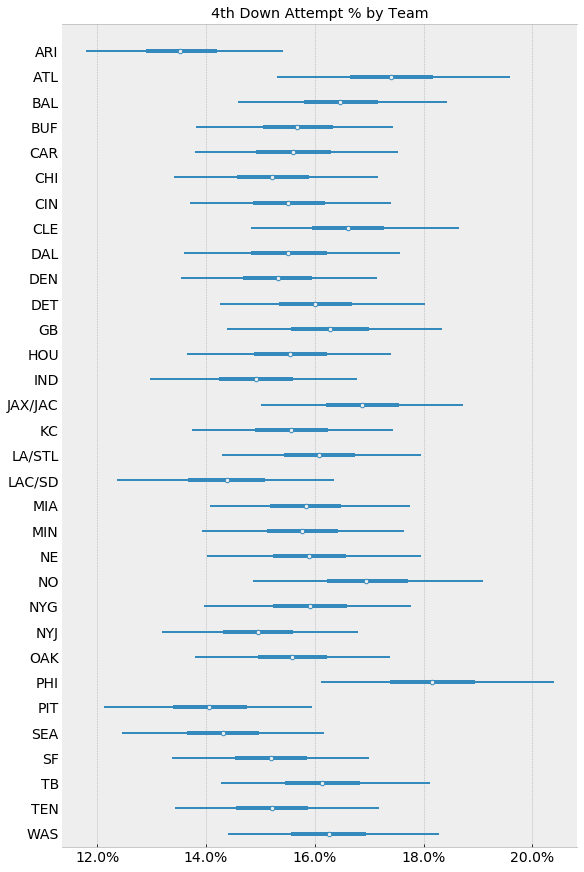
Again, even experimenting with stronger regularization via our priors, we don’t observe a lot of shrinkage of estimates towards the mean for those teams further away from the group, but we do note it for the stronger and weaker teams:

Weekly Model

For our last model expansion, we’ll look at whether being earlier or later in the season affects how aggressive teams are on fourth down.

Thus, for this model, we set up 17 priors for theta, again partially pooled:

Model Critique

The group mean, estimated via phi looks even more cohesive than previous model, suggesting lower variability from week to week.

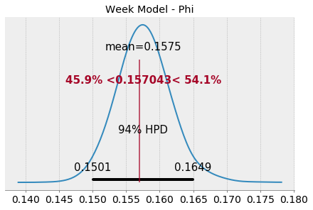
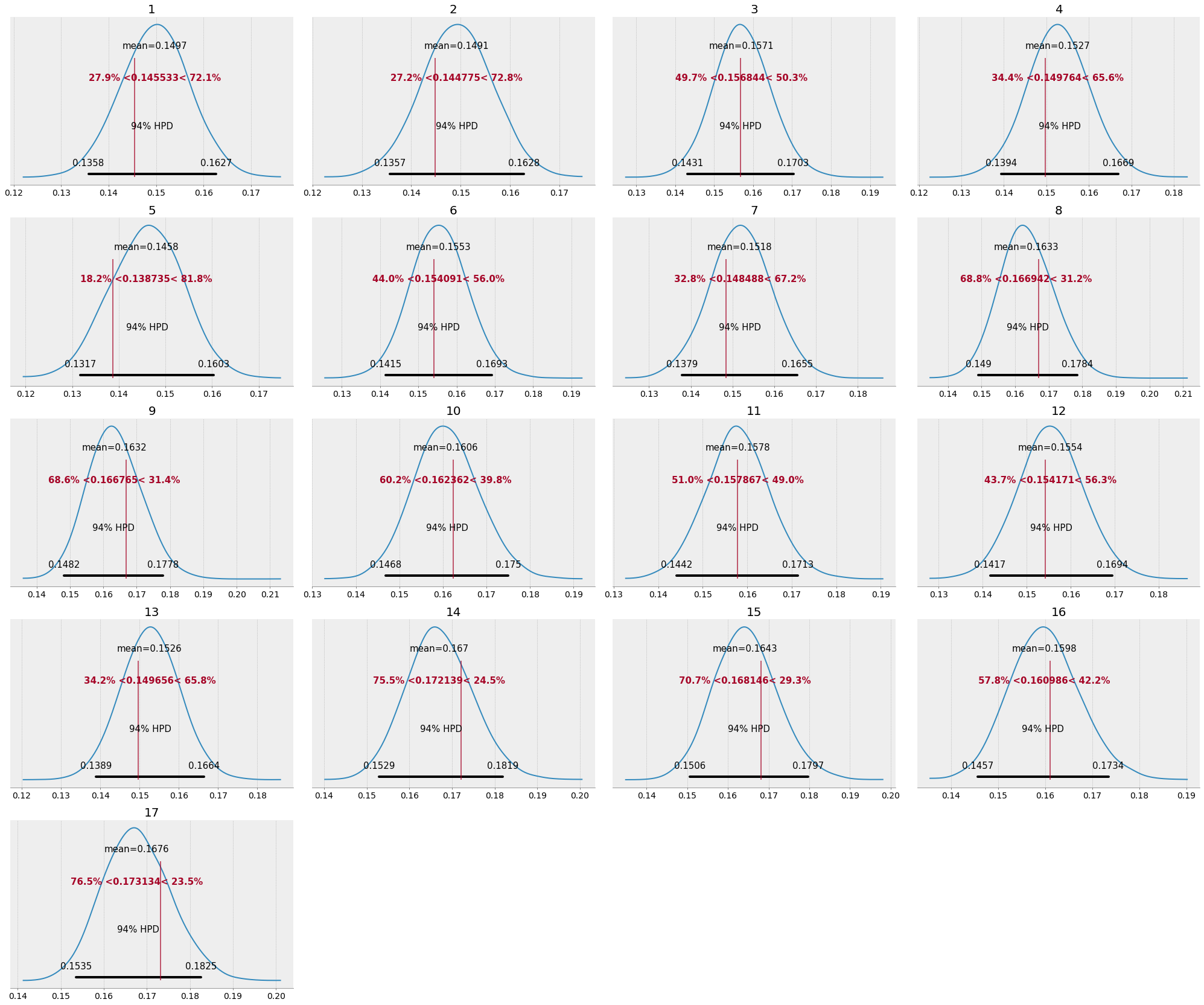
However, looking at theta by week, we can spot a slight upward trend from early weeks to week later in the regular season:

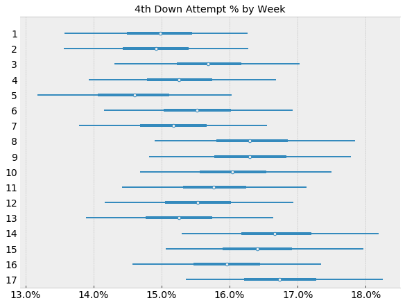
[Let’s come back to this trend at the end of the post.]

In this model, we can visually observe more shrinkage, particularly for weeks 5, 14, 15, and 17. This gives us some confidence that an un-pooled model, or non-Bayesian approach, would have likely under/overestimated the latent fourth down attempt %.

Weekly Trend Model

To check whether the upward trend we saw in our weekly model is quantifiable, let’s set up a quick linear model. If there is in fact a positive trend in fourth attempt % as the weeks progress, we should be able to estimate a positive slope/coefficient for week as a regressor.

Our model will be: $Y = \alpha + X\beta + \epsilon$

Where $X$ is a single feature vector made up of only week.

Assuming df_week is a dataframe with fourth downs attempt % computed by week of the season across all 11 seasons, we can set up a simple linear model like so:

with pm.Model() as attempts_week_linear_model:
    
    α = pm.Normal("α", mu=0, sd=20)
    
    β = pm.Normal("β", mu=0, sd=20)
    
    σ = pm.HalfNormal("σ", sd=20)
    μ = α + β * df_week["season_week"]
     
    y_attempt_ratio = pm.Normal("y_attempt_ratio", mu=μ, sd=σ, observed=df_week["fourth_down_attempt_pct"])

This is not a particularly complex model, nor does it need to be. We just want to estimate a simple slope parameter to confirm whether there is a positive relationship between “season_week” and the % of fourth downs attempted.

After sampling with MCMC/Nuts, we get the following parameter estimates, summarized for us by PyMC3:

      | mean    | sd      | hpd_3%  | hpd_97% |
|-----|---------|---------|---------|---------|
| α   | 0.14444 | 0.00433 | 0.13600 | 0.15235 |
| β   | 0.00140 | 0.00042 | 0.00060 | 0.00218 |
| σ   | 0.00831 | 0.00170 | 0.00537 | 0.00546 |

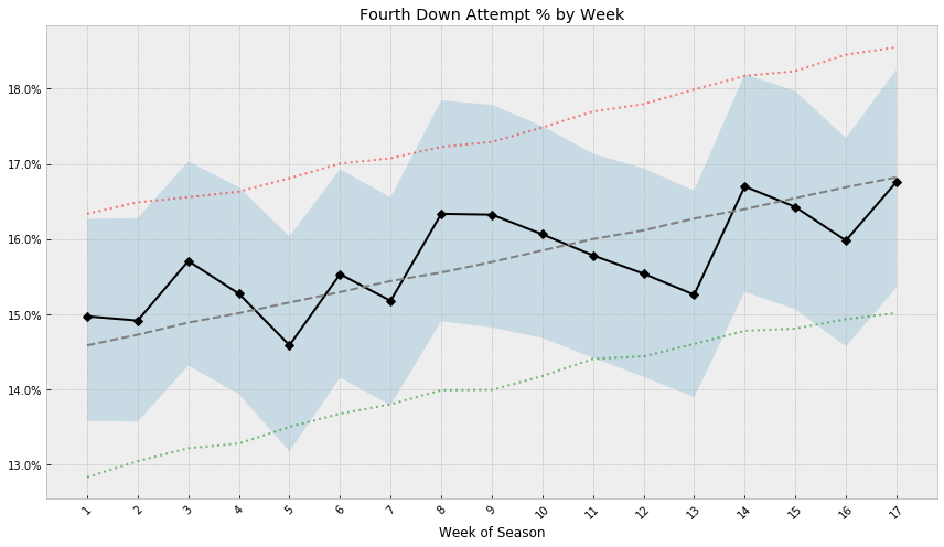
We’ll notice that the posterior for our slope parameter $\beta$, while small, is positive across the HPD interval. This implies that there is an average increase of fourth downs attempted of 0.14% per week, over the baseline average of 14.44%.

Plotting estimates for mean and HPD interval from our earlier model by week, along with the posterior predictive values from this model, we get visual confirmation of the upward trend. It’s also a nice check that we get sensible results from both models.

Model Evaluation and Comparison

While we’ve learned a lot about our data, and Bayesian model by building 4 separate models (from the same dataset, modeling the same outcome variable), we may have to pick one of the models. For example, if we wanted to predict fourth down attempts, we want to chose the model that best captures our data generating process.

In Bayesian modeling, there are a number of techniques and metrics to quantify model performance and to compare models.

PyMC3 and Arviz have some of the most effective approaches built in. For example, the aptly named “Widely Applicable Information Criterion”¹³, or WAIC, is a method for

estimating pointwise out-of-sample prediction accuracy from a fitted Bayesian model using the log-likelihood evaluated at the posterior simulations of the parameter values.⁹

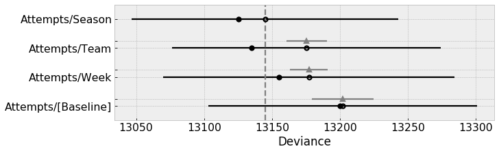
Lower values of WAIC are better, thus, for predictive accuracy, we would favor our season model:

| model               | rank | waic    | p_waic  | d_waic  | weight     | se      | dse     | warning | waic_scale |
|---------------------|------|---------|---------|---------|------------|---------|---------|---------|------------|
| Attempts/Season     | 0    | 13144.9 | 9.83728 | 0       | 0.969701   | 95.8144 | 0       | False   | deviance   |
| Attempts/Team       | 1    | 13175.4 | 20.1258 | 30.488  | 0.0178665  | 96.5892 | 14.8302 | False   | deviance   |
| Attempts/Week       | 2    | 13177.1 | 10.9837 | 32.1923 | 0.00689369 | 105.532 | 14.0059 | False   | deviance   |
| Attempts/[Baseline] | 3    | 13202   | 1.11554 | 57.0702 | 0.00553901 | 96.9478 | 22.772  | False   | deviance   |

It’s also good to see that our baseline model scores the worst of the four, confirming our initial take that the fully pooled model fails to capture our data well.

Further areas of exploration

I hope this was a helpful introduction to modeling with PyMC3. There are clearly a number of interesting avenues to pursue with this dataset.

As alluded to earlier, another way to expand on these models would be to introduce more domain knowledge about fourth down attempts in the model, similar to how Andrew Gelman introduced progressively more putting domain knowledge in the post referenced above.

We kept it very simple in our models so far, focusing on only one group/predictor at a time. Natural areas of model expansion would be to introduce other variables, or potentially create additional levels of hierarchy in our multi-level models.

One obvious metric to follow up fourth down conversion conversion is third down conversions, as teams that are better on third down will perhaps not get as many chances on fourth and may also not need to be as aggressive when they do get to fourth.

In addition, Bayesian modeling seems to be well suited to analyze a number of other key NFL stats, such as Passer Rating, which we’ll be taking a look at in a future post.

As always, please let me know if you have any comments or questions about this post.

Notes

1. NFL teams are getting smarter, and better, on fourth downs ↩

2. New York Times 4th Down Bot (sadly, the accompanying Twitter account seems to have stopped posting some time in 2017…) ↩

3. nflscrapR-data Github repo ↩

4. NFLScraperR library for R ↩

5. What exactly is a Bayesian model? ↩

6. Statistical Rethinking: A Bayesian Course with Examples in R and Stan ↩

7. Model building and expansion for golf putting ↩

8. https://docs.pymc.io/api/stats.html ↩

9. Practical Bayesian model evaluation using leave-one-out cross-validation and WAIC ↩ ↩²

10. Towards A Principled Bayesian Workflow and also the related paper, Toward a principled Bayesian workflow in cognitive science, as well as Visualization in Bayesian workflow ↩

11. A Primer on Bayesian Methods for Multilevel Modeling ↩

12. Hierarchical Partial Pooling ↩

13. also known as “Watanabe–Akaike information criterion” ↩