Dice, Polls & Dirichlet Multinomials

This post is also available as a Jupyter Notebook on Github.

As part of a longer term project to learn Bayesian Statistics, I’m currently reading Bayesian Data Analysis, 3rd Edition by Andrew Gelman, John Carlin, Hal Stern, David Dunson, Aki Vehtari, and Donald Rubin, commonly known as BDA3. Although I’ve been using Bayesian statistics and probabilistic programming languages, like PyMC3, in projects for the last year or so, this book forces me to go beyond a pure practitioner’s approach to modeling, while still delivering very practical value.

Below are a few take always from the earlier chapters in the book I found interesting. They are meant to hopefully inspire others to learn about Bayesian statistics, without trying to be overly formal about the math. If something doesn’t look 100% to the trained mathematicians in the room, please let me know, or just squint a little harder. ;)

We’ll cover:

• Some common conjugate distributions
• An example of the Dirichlet-Multinomial distribution using dice rolls
• Two examples involving polling data from BDA3

Conjugate Distributions

In Chapter 2 of the book, the authors introduce several choices for prior probability distributions, along with the concept of conjugate distributions in section 2.4.

From Wikipedia

In Bayesian probability theory, if the posterior distributions p(θ | x) are in the same probability distribution family as the prior probability distribution p(θ), the prior and posterior are then called conjugate distributions, and the prior is called a conjugate prior for the likelihood function

John Cook has this helpful diagram on his website that shows some common families of conjugate distributions:

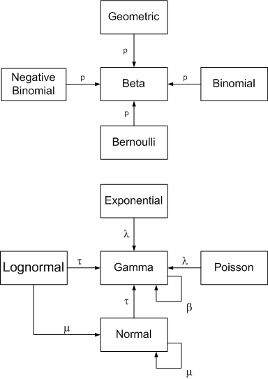
Conjugate distributions are a very important concept in probability theory, owing to a large degree to some nice mathematical properties that make computing the posteriors more tractable. Even with increasingly better computational tools, such as MCMC, models based on conjugate distributions are advantageous.

Beta-Binomial

One of the better known examples of conjugate distributions is the Beta-Binomial distribution, which is often used to model series of coin flips (the ever present topic in posts about probability).

While the Binomial distribution represents the probability of success in a series of Bernoulli trials, the Beta distribution here represents the prior probability distribution of the probability of success for each trial.

Thus, the probability $p$ of a coin landing on head is modeled to be Beta distributed (with parameters $\alpha$ and $\beta$), while the likelihood of heads and tails is assumed to follow a Binomial distribution with parameters $n$ (representing the number of flips) and the Beta-distributed $p$, thus creating the link.

\[p \sim Beta(\alpha, \beta)\] \[y \sim Binomial(n, p)\]

Gamma-Poisson

Another often-used conjugate distribution is the Gamma-Poisson distribution, so named because the rate parameter $\lambda$ that parameterizes the Poisson distribution is modeled as a Gamma distribution:

\[\lambda \sim Gamma(k, \theta)\] \[y \sim Poisson(\lambda)\]

While the discrete Poisson distribution is often used in applications of count data, such as store customers, eCommerce orders, website visits, the Gamma distribution serves as a useful distribution to model the rate at which these events occur ($\lambda$), since the Gamma distribution models positive continuous values only, but is otherwise quite flexible in its parameterization:

This distribution is also known as the Negative-Binomial distribution, which we can think of as a mixture of Poission distributions.

If you find this confusing, you’re not alone, and maybe you’ll start to appreciate why so often we try to approximate things using the good old Normal distribution…

Dirichlet-Multinomial

A perhaps even more interesting yet seemingly less talked-about example of conjugate distributions is the Dirichlet-Multinomial distribution, introduced in chapter 3 of BDA3.

One way of think about the Dirichlet-Multinomial distribution is that while the Multinomial (i.e. multiple choices) distribution is a generalization of the Binomial distribution (i.e. binary choice), the Dirichlet distribution is a generalization of the Beta distribution. That is, while the Beta distribution models the probability of a single probability $p$, the Dirichlet models the probabilities of multiple, mutually exclusive choices, parameterized by $a$ which is referred to as the concentration parameter and represents the weights for each choice (we’ll see more on that later).

In other words, think of coins for the Beta-Binomial distribution and dice for the Dirichlet-Multinomial distribution.

\[\theta \sim Dirichlet(a)\] \[y \sim Multinomial(n, \theta)\]

In the wild, we might encounter the Dirichlet distribution these days often in the context of topic modeling in natural language processing, where it’s commonly used as part of a Latent Dirichlet Allocation (or LDA) model, which is a fancy way of saying we’re trying to figure out the probability of an article belonging to a certain topic given its content.

However, for our purposes, let’s look at the Dirichlet-Multinomial in the context of simple multiple choices, and let’s start by throwing dice as a motivating example:

Throwing Dice

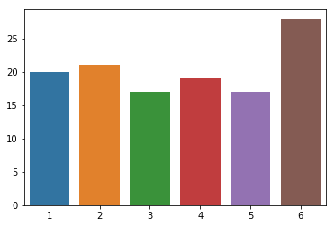
Let’s first create some data representing 122 rolls of six-sided die, where $p$ represents the expected probability for each side of a fair die, i.e. $1/6$

y = np.asarray([20,  21, 17, 19, 17, 28])
k = len(y)
p = 1/k
n = y.sum()

n, p

(122, 0.16666666666666666)

Just looking at a simple bar plot of the data, we suspect that we might not be dealing with a fair die!

sns.barplot(x=np.arange(1, k+1), y=y);

However, students of Bayesian statistics that we are, we’d like to go further and quantify our uncertainty in the fairness of the die and calculate the probability that someone slipped us loaded dice.

Let’s set up a simple model in PyMC3 that not only calculates the posterior probability for $theta$ (i.e. the probability for each side of the die), but also estimates the die’s bias for returning a $6$. We will use a Deterministic variable for that purpose, in addition to our unobserved (theta) and observed (results) random variables.

For the prior on $theta$, we’ll assume a non-informative Uniform distribution, by initializing the Dirichlet prior with a series of 1s for the parameter a, one for each of the k possible outcomes. This is similar to initializing a Beta distribution as $Beta(1, 1)$, which corresponds to the Uniform distribution (more on this here).

with pm.Model() as dice_model:
    
    # initializes the Dirichlet distribution with a uniform prior:
    a = np.ones(k) 
    
    theta = pm.Dirichlet("theta", a=a)
    
    # Since theta[5] will hold the posterior probability of rolling a 6
    # we'll compare this to the reference value p = 1/6
    six_bias = pm.Deterministic("six_bias", theta[k-1] - p)
    
    results = pm.Multinomial("results", n=n, p=theta, observed=y)

Starting with version 3.5, PyMC3 includes a handy function to plot models in plate notation:

pm.model_to_graphviz(dice_model)

Let’s draw 1,000 samples from the joint posterior using the default NUTS sampler:

with dice_model:
    dice_trace = pm.sample(draws=1000)

Auto-assigning NUTS sampler...
Initializing NUTS using jitter+adapt_diag...
Multiprocess sampling (4 chains in 4 jobs)
NUTS: [theta]
Sampling 4 chains: 100%|██████████| 6000/6000 [00:01<00:00, 3822.31draws/s]

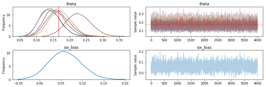
From the traceplot, we can already see that one of the $theta$ posteriors isn’t in line with the rest:

with dice_model:
    pm.traceplot(dice_trace, combined=True, lines={"theta": p})

We’ll plot the posterior distributions for each $theta$ and compare it our reference value $p$ to see if the 95% HPD (Highest Posterior Density) interval includes $p = 1/6$.

axes = pm.plot_posterior(dice_trace, varnames=["theta"], ref_val=np.round(p, 3))
for i, ax in enumerate(axes):
    ax.set_title(f"{i+1}")

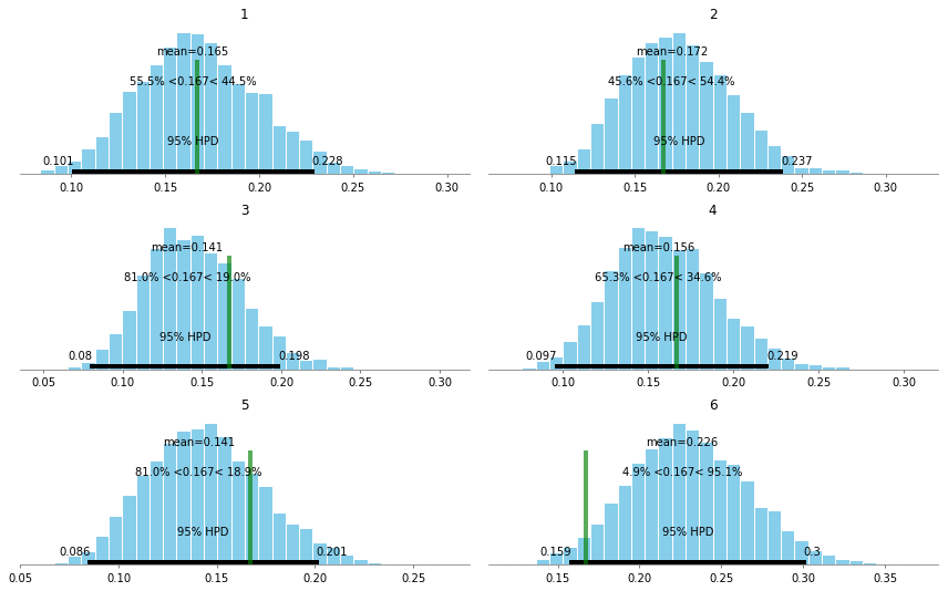
We can clearly see that the HPD for the posterior probability for rolling a $6$ barely includes the value we’d expect from a fair die.

To be more precise, let’s plot the probability of our die being biased towards $6$, by comparing $theta[Six]$ to $p$

ax = pm.plot_posterior(dice_trace, varnames=["six_bias"], ref_val=[0])
ax.set_title(f"P(Theta[Six] - {p:.2%})");

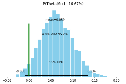
Lastly, we can calculate the probability that the die is biased towards $6$ by calculating the density to the right of our reference line at $0$:

six_bias_perc = len(dice_trace["six_bias"][dice_trace["six_bias"]>0])/len(dice_trace["six_bias"])
      
print(f'P(Six is biased) = {six_bias_perc:.2%}')

P(Six is biased) = 95.25%

Thus, there’s a better than 95% chance that our die is biased towards $6$. Better get some new dice…!

Polling #1

Let’s turn our review of the Dirichlet-Multinomial distribution to another example, concerning polling data.

In section 3.4 of BDA3 on multivariate models and, specifically the section on Multinomial Models for Categorical Data, the authors include a, little dated, example of polling data in the 1988 Presidential race between George H.W. Bush and Michael Dukakis.

Spoiler alert for those not following politics back then: Bush won by a huge margin. Since 1988, no candidate in a Presidential election has managed to equal or surpass Bush’s share of the electoral or popular vote.

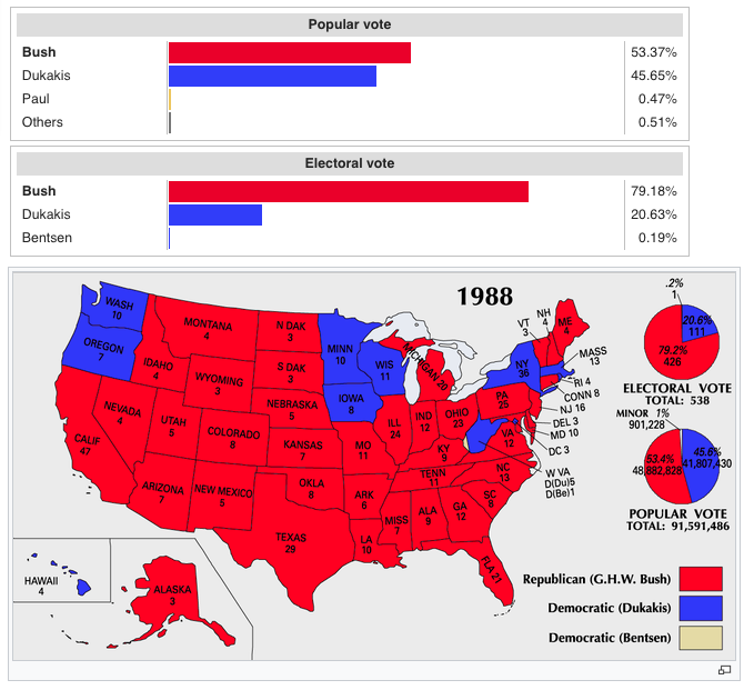
(Image credit: https://commons.wikimedia.org/wiki/File:ElectoralCollege1988-Large.png)

Anyway, back to the data problem! Here’s the setup:

• 1,447 likely voters were surveyed about their preferences in the upcoming presidential election
• Their responses were:
  • Bush: 727
  • Dukakis: 583
  • Other: 137
• What is the probability that more people will vote for Bush over Dukakis?
  • i.e. what is the difference in support for the two major candidates?

We set up the data, where $k$ represents the number of choices the respondents had:

y = np.asarray([727, 583, 137])
n = y.sum()
k = len(y)

We, again, set up a simple Dirichlet-Multinomial model and include a Deterministic variable that calculates the value of interest - the difference in probability of respondents for Bush vs. Dukakis.

with pm.Model() as polling_model:
    
    # initializes the Dirichlet distribution with a uniform prior:
    a = np.ones(k) 
    
    theta = pm.Dirichlet("theta", a=a)
    
    bush_dukakis_diff = pm.Deterministic("bush_dukakis_diff", theta[0] - theta[1])
    
    likelihood = pm.Multinomial("likelihood", n=n, p=theta, observed=y)

pm.model_to_graphviz(polling_model)

with polling_model:
    polling_trace = pm.sample(draws=1000)

Looking at the % difference between respondents for Bush vs Dukakis, we can see that most of the density is greater than 0%, signifying a strong advantage for Bush in this poll.

We’ve also fit a $Beta$ distribution to this data via scipy.stats, and we can see that the posterior of the difference of the 2 $theta$ values fits a Beta distribution very nicely (which is to be expected given the properties of the Dirichlet distribution as a multivariate generalization of the Beta distribution).

_, ax = plt.subplots(1,1, figsize=(10, 6))
sns.distplot(polling_trace["bush_dukakis_diff"], bins=20, ax=ax, kde=False, fit=stats.beta)
ax.axvline(0, c='g', linestyle='dotted')
ax.set_title("% Difference Bush vs Dukakis")
ax.set_xlabel("% Difference");

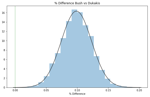
Percentage of samples with bush_dukakis_diff > 0:

bush_dukakis_diff_perc = len(polling_trace["bush_dukakis_diff"][polling_trace["bush_dukakis_diff"]>0])/len(polling_trace["bush_dukakis_diff"])
      
print(f'P(More Responses for Bush) = {bush_dukakis_diff_perc:.0%}')

P(More Responses for Bush) = 100%

Polling #2

As an extension to the previous model, the authors of BDA include an exercise in chapter 3.10 (Exercise 2) that presents us with polling data from the 1988 Presidential race, taking before and after the one of the debates.

Comparison of two multinomial observations: on September 25, 1988, the evening of a presidential campaign debate, ABC News conducted a survey of registered voters in the United States; 639 persons were polled before the debate, and 639 different persons were polled after. The results are displayed in Table 3.2. Assume the surveys are independent simple random samples from the population of registered voters. Model the data with two different multinomial distributions. For $j = 1, 2$, let $\alpha_j$ be the proportion of voters who preferred Bush, out of those who had a preference for either Bush or Dukakis at the time of survey $j$. Plot a histogram of the posterior density for $\alpha_2 − \alpha_1$. What is the posterior probability that there was a shift toward Bush?

Let’s copy the data from the exercise and model the problem as a probabilistic model, again using PyMC3:

data = pd.DataFrame([
        {"candidate": "bush", "pre": 294, "post": 288},
        {"candidate": "dukakis", "pre": 307, "post": 332},
        {"candidate": "other", "pre": 38, "post": 10}
       ], columns=["candidate", "pre", "post"])

	candidate	pre	post
0	bush	294	288
1	dukakis	307	332
2	other	38	10

Convert to 2x3 array:

y = data[["pre", "post"]].T.values
y

array([[294, 307,  38],
       [288, 332,  10]])

Number of respondents in each survey:

n = y.sum(axis=1) 
n

array([639, 630])

Number of respondents for the 2 major candidates in each survey:

m = y[:, :2].sum(axis=1) 
m

array([601, 620])

For this model, we’ll need to set up the priors slightly differently. Instead of 1 set of thetas, we need 2, one for each survey (pre/post debate). To do that without creating specific pre/post versions of each variable, we’ll take advantage of PyMC3’s shape parameter, available for most (all?) distributions.

In this case, we’ll need a 2-dimensional shape parameter, representing the number of debates n_debates and the number of choices in candidates n_candidates

n_debates, n_candidates = y.shape
n_debates, n_candidates

(2, 3)

Thus, we need to initialize a Dirichlet distribution prior with shape (2,3) and then refer to the relevant parameters by index where needed.

with pm.Model() as polling_model_debates:
    
    # initializes the Dirichlet distribution with a uniform prior:
    shape = (n_debates, n_candidates)
    a = np.ones(shape)
    
    # This creates a separate Dirichlet distribution for each debate
    # where sum of probabilities across candidates = 100% for each debate
    theta = pm.Dirichlet("theta", a=a, shape=shape)
    
    # get the "Bush" theta for each debate, at index=0
    # and normalize across supporters for the 2 major candidates
    bush_pref = pm.Deterministic("bush_pref", theta[:, 0] * n / m)
    
    # to calculate probability that support for Bush shifted from debate 1 [0] to 2 [1]
    bush_shift = pm.Deterministic("bush_shift", bush_pref[1]-bush_pref[0])
    
    # because of the shapes of the inputs, this essentially creates 2 multinomials, 
    # one for each debate
    responses = pm.Multinomial("responses", n=n, p=theta, observed=y)

For models with multi-dimensional shapes, it’s always good to check the shapes of the various parameters before sampling:

for v in polling_model_debates.unobserved_RVs:
    print(v, v.tag.test_value.shape)

theta_stickbreaking__ (2, 2)
theta (2, 3)
bush_pref (2,)
bush_shift ()

The plate notation visual can also help with that:

pm.model_to_graphviz(polling_model_debates)

Let’s sample with a slightly higher number of draws and tuning steps:

with polling_model_debates:
    polling_trace_debates = pm.sample(draws=3000, tune=1500)

A quick look at the traceplot to make sure the model converged smoothly:

with polling_model_debates:
    pm.traceplot(polling_trace_debates, combined=True)

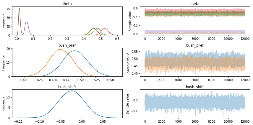
Let’s take a look at the means of the posteriors for theta, indicating the % of support for each candidate pre & post debate:

s = ["pre", "post"]
candidates = data["candidate"].values
pd.DataFrame(polling_trace_debates["theta"].mean(axis=0), index=s, columns=candidates)

	bush	dukakis	other
pre	0.459702	0.479663	0.060635
post	0.456571	0.526066	0.017362

Just from the means, we can see that the number of Bush supporters has likely decreased post debate from 48.8% to 46.3% (as a % of supporters of the 2 major candidates):

pd.DataFrame(polling_trace_debates["bush_pref"].mean(axis=0), index=s, columns=["bush_pref"])

	bush_pref
pre	0.488768
post	0.463935

Let’s compare the results visually, by plotting the posterior distributions of the pre/post debate values for % responses for Bush and the posterior for pre/post difference in Bush supporters:

_, ax = plt.subplots(2,1, figsize=(10, 10))

sns.distplot(polling_trace_debates["bush_pref"][:,0], hist=False, ax=ax[0], label="Pre-Debate")
sns.distplot(polling_trace_debates["bush_pref"][:,1], hist=False, ax=ax[0], label="Post-Debate")
ax[0].set_title("% Responses for Bush vs Dukakis")
ax[0].set_xlabel("% Responses");

sns.distplot(polling_trace_debates["bush_shift"], hist=True, ax=ax[1], label="P(Bush Shift)")
ax[1].axvline(0, c='g', linestyle='dotted')
ax[1].set_title("% Shift Pre/Prior Debate")
ax[1].set_xlabel("% Shift");

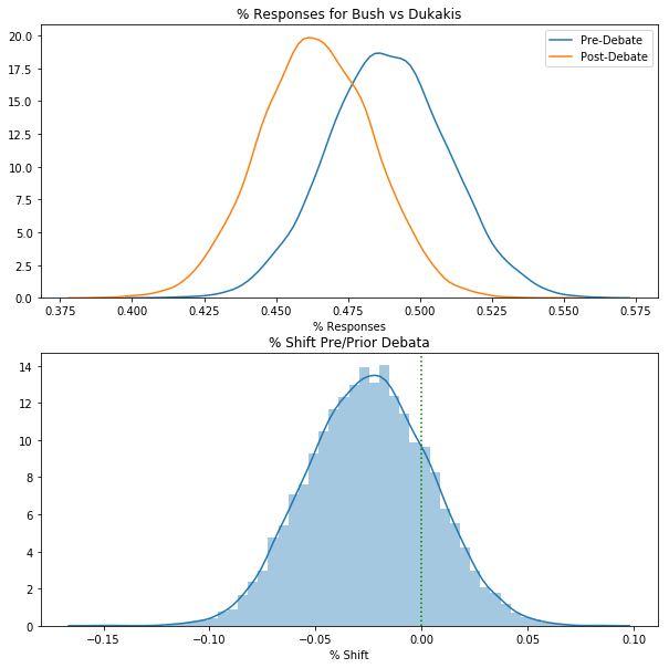
From the second plot, we can already see that a large portion of the posterior density is below 0, but let’s be precise and actually calculate the probability that support shifted towards Bush after the debate:

perc_shift = (len(polling_trace_debates["bush_shift"][polling_trace_debates["bush_shift"] > 0])
              /len(polling_trace_debates["bush_shift"])
             )
print(f'P(Shift Towards Bush) = {perc_shift:.1%}')

P(Shift Towards Bush) = 19.9%

While that was a sort of round-about way to show that Bush lost support during the September debate, hopefully this illustrated the flexibility and robustness of probabilistic models (and PyMC3).

If you have any thoughts or feedback on this post, please let me know!

This post is also available as a Jupyter Notebook on Github.