
Exploring Google BigQuery with the R tidyverse
In recent years, R has made quite the comeback in statistics and data science, largely thanks to a new collection of easy-to-use, yet powerful packages known as the tidyverse. These packages, primarily dplyr and ggplot make data wrangling and visualizing intuitive and fun, even for newcomers to data science. Not only that, they’re robust and powerful for advanced analytics and are employed in many production settings. In this post, we’ll take a look at using packages from the R tidyverse to query and visually explore data in Google BigQuery. We’ll primarily use dplyr and the slightly confusingly named dbplyr packages.
Libraries
Aside from the main tidyverse package, you’ll need the following libraries to make this work, most notably dbplyr, bigrquery and DBI to handle database connections. We’ll also pick an hrbrthemes theme for the ggplot plots.
library(tidyverse)
library(dbplyr)
library(bigrquery)
library(DBI)

library(hrbrthemes)

theme_set(hrbrthemes::theme_ipsum_rc())
BigQuery Connection
First, we need to set up a connection object to BigQuery we can use for our queries. We will use a service account to authenticate, although you can also use interactive, browser-based authentication.
bq_auth(
  path = "<path-to-your-bigquery-service-account>.json"
)

con <- dbConnect(
  bigrquery::bigquery(),
  project = "<your_project>",
  dataset = "<your_dataset>",
  billing = "<your_billing_project>"
)
For this post, we’ll use the NFL Play-by-Play dataset we’ve seen before when I wrote about the nfl-dbt repo back in December, but you can use any dataset you have in BigQuery to apply these techniques.
After we’ve set up the connection object con, we’ll create references to tables in our dataset. We can use glimpse to take a quick look at our data. Notice that we don’t query anything until we actually call glimpse. It only issues a quick metadata query and selects a few rows from BigQuery, as indicated by the line Rows: ?? at the top. In fact, we will not find any billable query in our Query History log for this call, it seems this is analogous to the preview functionality in the bigquery UI - so we’ll want to prefer glimpse over something like head for BigQuery.
games <- tbl(con, "games")
plays <- tbl(con, "plays")

glimpse(games)
## Rows: ??
## Columns: 13
## Database: BigQueryConnection
## $ season_code      <chr> "REG2011", "REG2017", "REG2011", "REG2011", "REG2011…
## $ game_id          <int> 2011120500, 2017120400, 2012010113, 2012010107, 2012…
## $ game_date        <date> 2011-12-05, 2017-12-04, 2012-01-01, 2012-01-01, 201…
## $ season_nbr       <int> 2011, 2017, 2011, 2011, 2011, 2011, 2011, 2011, 2011…
## $ season_type_code <chr> "REG", "REG", "REG", "REG", "REG", "REG", "REG", "RE…
## $ week_nbr         <int> 13, 13, 17, 17, 17, 17, 17, 17, 17, 17, 17, 17, 17, …
## $ home_team_code   <chr> "JAC", "CIN", "DEN", "PHI", "JAC", "CLE", "NYG", "MI…
## $ away_team_code   <chr> "SD", "PIT", "KC", "WAS", "IND", "PIT", "DAL", "NYJ"…
## $ home_score       <int> 14, 20, 3, 34, 19, 9, 31, 19, 45, 13, 23, 49, 22, 45…
## $ away_score       <int> 38, 23, 7, 10, 13, 13, 14, 17, 17, 17, 20, 21, 23, 2…
## $ game_url         <chr> "http://www.nfl.com/liveupdate/game-center/201112050…
## $ dbt_batch_id     <chr> "76b60fbb-c0e0-42aa-a694-d95d82b436ee", "76b60fbb-c0…
## $ dbt_batch_ts     <dttm> 2020-02-11 14:29:52, 2020-02-11 14:29:52, 2020-02-1…
Querying BigQuery data using dplyr
Next, we can use standard dplyr verbs like filter or select against our games table object, which dbplyr will translate into BigQuery-compatible SQL.
Notice that since we are not assigning this query to an object, we are executing the query right away to print the results to the console:
games %>%
  filter(starts_with(season_code, "REG")) %>%
  select(season_code, everything(), -starts_with("dbt"), -ends_with("score"), -game_id, -game_url)
## # Source:   lazy query [?? x 7]
## # Database: BigQueryConnection
##    season_code game_date  season_nbr season_type_code week_nbr home_team_code
##    <chr>       <date>          <int> <chr>               <int> <chr>
##  1 REG2013     2013-12-16       2013 REG                    15 DET
##  2 REG2011     2011-09-08       2011 REG                     1 GB
##  3 REG2015     2015-11-09       2015 REG                     9 SD
##  4 REG2012     2012-12-02       2012 REG                    13 NYJ
##  5 REG2012     2012-12-02       2012 REG                    13 STL
##  6 REG2012     2012-12-02       2012 REG                    13 GB
##  7 REG2012     2012-12-02       2012 REG                    13 BUF
##  8 REG2012     2012-12-02       2012 REG                    13 SD
##  9 REG2012     2012-12-02       2012 REG                    13 OAK
## 10 REG2012     2012-12-02       2012 REG                    13 KC
## # … with more rows, and 1 more variable: away_team_code <chr>
If we were to instead assign the query to an object, no query will get executed unless we call one of the query execution functions. That is, we’ve constructed a lazy query object. This is in some ways similar to how a query engine like SparkSQL might create a query execution graph.
reg_season <- games %>%
  filter(starts_with(season_code, "REG")) %>%
  select(season_code, everything(), -starts_with("dbt"), -ends_with("score"), -game_id, -game_url)
To actually run this query, we will need to use one of the functions like collect(), or head() to force query execution. However, before we do that, we can still add query statements to our object, which will be part of the query when it’s finally executed. This is a really nice option if we need to logically break up query construction, without incurring additional BigQuery processing costs.
reg_season %>%
  arrange(game_date) %>%
  collect()
## # A tibble: 2,816 x 7
##    season_code game_date  season_nbr season_type_code week_nbr home_team_code
##    <chr>       <date>          <int> <chr>               <int> <chr>
##  1 REG2009     2009-09-10       2009 REG                     1 PIT
##  2 REG2009     2009-09-13       2009 REG                     1 SEA
##  3 REG2009     2009-09-13       2009 REG                     1 ATL
##  4 REG2009     2009-09-13       2009 REG                     1 IND
##  5 REG2009     2009-09-13       2009 REG                     1 CIN
##  6 REG2009     2009-09-13       2009 REG                     1 GB
##  7 REG2009     2009-09-13       2009 REG                     1 NYG
##  8 REG2009     2009-09-13       2009 REG                     1 ARI
##  9 REG2009     2009-09-13       2009 REG                     1 HOU
## 10 REG2009     2009-09-13       2009 REG                     1 BAL
## # … with 2,806 more rows, and 1 more variable: away_team_code <chr>
Notice that the R console also gives us the relevant job id and information about billable bytes:
Running job 'nfl-pbp.job_xIelG7P_Hhjm8DUm1D3s9RajsXEt.US' [|]  1s
Complete
Billed: 10.49 MB
Downloading 2,816 rows in 1 pages.
More Advanced Query Options
Let’s take a look at a few more ways we can query this data using dplyr. The mutate function is one of the more powerful function in the tidyverse to embed logic in your queries. You can use it to create new columns and/or override existing columns. In the example below, we’ll create a few logical columns. Note how you refer to columns you’ve created within the same mutate function. This is similar to how data warehouse platforms like Snowflake implement lateral aliasing, which, ironically, isn’t available in BigQuery. Note that we can also use the mutate stament multiple times in the same operation.
The case_when function operates much like its SQL equivalent case when as we’ll see below.
team_code <- "SEA"
team_name <- "Seattle"

team_games <- games %>%
  mutate(
      is_team_home_game = home_team_code == team_code,
      is_team_away_game = away_team_code == team_code,
      is_team_game = is_team_home_game == TRUE | is_team_away_game == TRUE
      ) %>%
  filter(
    season_nbr >= 2015,
    starts_with(season_code, "REG"),
    is_team_game == TRUE
  ) %>%
  mutate(team_win = case_when(
            is_team_home_game & home_score > away_score ~ TRUE,
            is_team_away_game & away_score > home_score ~ TRUE,
            TRUE ~ FALSE
          ),
         team_spread_home = case_when(
           is_team_home_game == TRUE ~ home_score - away_score,
           TRUE ~ 0)
  ) %>%
  select(season_code, game_date, home_team_code, away_team_code, is_team_home_game, team_spread_home) %>%
  arrange(game_date)
Passing the unexecuted query object to show_query() allows us to take a peak at the generated query before submitting it to BigQuery. Noticed how dbplyr translates query steps into subqueries and case_when into case when.
team_games %>% show_query()
## <SQL>
## SELECT `season_code`, `game_date`, `home_team_code`, `away_team_code`, `is_team_home_game`, CASE
## WHEN (`is_team_home_game` = TRUE) THEN (`home_score` - `away_score`)
## ELSE (0.0)
## END AS `team_spread_home`
## FROM (SELECT `season_code`, `game_id`, `game_date`, `season_nbr`, `season_type_code`, `week_nbr`, `home_team_code`, `away_team_code`, `home_score`, `away_score`, `game_url`, `dbt_batch_id`, `dbt_batch_ts`, `is_team_home_game`, `is_team_away_game`, `is_team_home_game` = TRUE OR `is_team_away_game` = TRUE AS `is_team_game`
## FROM (SELECT `season_code`, `game_id`, `game_date`, `season_nbr`, `season_type_code`, `week_nbr`, `home_team_code`, `away_team_code`, `home_score`, `away_score`, `game_url`, `dbt_batch_id`, `dbt_batch_ts`, `home_team_code` = 'SEA' AS `is_team_home_game`, `away_team_code` = 'SEA' AS `is_team_away_game`
## FROM `games`) `dbplyr_001`) `dbplyr_002`
## WHERE ((`season_nbr` >= 2015.0) AND (starts_with(`season_code`, 'REG')) AND (`is_team_game` = TRUE))
## ORDER BY `game_date`
We will store the query results in a local object so we can further manipulate it in R.
team_games <- team_games %>% collect() # <- executes the query
head(team_games, 20)
## # A tibble: 20 x 6
##    season_code game_date  home_team_code away_team_code is_team_home_ga…
##    <chr>       <date>     <chr>          <chr>          <lgl>
##  1 REG2015     2015-09-13 STL            SEA            FALSE
##  2 REG2015     2015-09-20 GB             SEA            FALSE
##  3 REG2015     2015-09-27 SEA            CHI            TRUE
##  4 REG2015     2015-10-05 SEA            DET            TRUE
##  5 REG2015     2015-10-11 CIN            SEA            FALSE
##  6 REG2015     2015-10-18 SEA            CAR            TRUE
##  7 REG2015     2015-10-22 SF             SEA            FALSE
##  8 REG2015     2015-11-01 DAL            SEA            FALSE
##  9 REG2015     2015-11-15 SEA            ARI            TRUE
## 10 REG2015     2015-11-22 SEA            SF             TRUE
## 11 REG2015     2015-11-29 SEA            PIT            TRUE
## 12 REG2015     2015-12-06 MIN            SEA            FALSE
## 13 REG2015     2015-12-13 BAL            SEA            FALSE
## 14 REG2015     2015-12-20 SEA            CLE            TRUE
## 15 REG2015     2015-12-27 SEA            STL            TRUE
## 16 REG2015     2016-01-03 ARI            SEA            FALSE
## 17 REG2016     2016-09-11 SEA            MIA            TRUE
## 18 REG2016     2016-09-18 LA             SEA            FALSE
## 19 REG2016     2016-09-25 SEA            SF             TRUE
## 20 REG2016     2016-10-02 NYJ            SEA            FALSE
## # … with 1 more variable: team_spread_home <dbl>
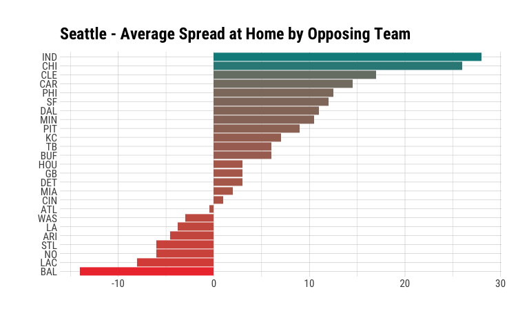
Since team_games is a tibble object, and not a query object, we can use R functions such as factor that would not have an equivalent in SQL:
team_home_games <- team_games %>%
  filter(is_team_home_game == TRUE) %>%
  mutate(home_team_code = factor(home_team_code),
         away_team_code = factor(away_team_code)) %>%
  group_by(away_team_code) %>%
  summarise(avg_spread_home = mean(team_spread_home))
Similarly, we can pass this tibble to ggplot to visualize our data:
ggplot(team_home_games,
            aes(x = avg_spread_home,
               y = reorder(away_team_code, avg_spread_home),
               fill = avg_spread_home,
               label = avg_spread_home)
            ) +
    geom_col(show.legend = FALSE) +
    scale_fill_continuous(low = "brown2",
                          high = "cyan4",
                          na.value = "grey50",
                          guide = "colourbar",
                          aesthetics = "fill") +
    labs(x = "", y = "") +
    ggtitle(str_c(team_name, "Average Spread at Home by Opposing Team", sep = " - "))
Fourth Downs
Let’s look at a few more ways to visualize this data, inspired by our look at Modeling of NFL Football Fourth Down Attempts a couple of months ago, to get an idea of how dplyr and dbplyr can fit into our statistical workflow.
First, we’ll take our plays data in BigQuery and filter to fourth down plays only, while also creating a few columns we’ll use in visualizations later. Note again that fourth_downs here does not yet hold any data locally, but is a collection of query instructions, yet to be executed.
fourth_downs <- plays %>%
    filter(down == 4, is_field_goal_attempt == FALSE) %>%
    mutate(team_code = off_team_code,
           season_type_code = str_to_lower(season_type_code),
           fourth_downs = 1,
           fourth_down_attempts = if_else(is_fourth_down_attempt == TRUE, 1, 0),
           fourth_down_conversions = if_else(is_fourth_down_converted == TRUE, 1, 0)) %>%
    select(play_id, season_nbr, season_type_code, team_code, fourth_downs,
           fourth_down_attempts, fourth_down_conversions)
Summarize by Season
season_sum_fourth_downs <- fourth_downs %>%
  group_by(season_nbr, season_type_code) %>%
  summarise(fourth_downs = sum(fourth_downs),
            fourth_down_attempts = sum(fourth_down_attempts),
            fourth_down_conversions = sum(fourth_down_conversions)) %>%
  collect() %>% # runs the query
  ungroup() %>% # post query from here on
  mutate(season_nbr = factor(season_nbr),
         season_type_code = factor(season_type_code))

glimpse(season_sum_fourth_downs)
## Rows: 33
## Columns: 5
## $ season_nbr              <fct> 2013, 2009, 2014, 2015, 2018, 2011, 2018, 201…
## $ season_type_code        <fct> reg, reg, post, post, pre, reg, reg, post, pr…
## $ fourth_downs            <dbl> 3181, 3183, 140, 151, 870, 3103, 2932, 134, 8…
## $ fourth_down_attempts    <dbl> 465, 553, 24, 30, 152, 426, 532, 27, 124, 588…
## $ fourth_down_conversions <dbl> 224, 279, 15, 15, 74, 185, 300, 11, 55, 285, …
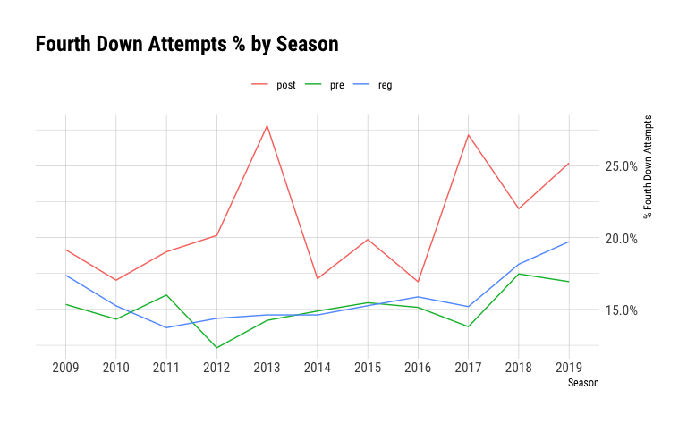
Plot % Attempts by Season
ggplot(season_sum_fourth_downs,
       aes(x=season_nbr,
           y=fourth_down_attempts/fourth_downs,
           group=season_type_code,
           color=season_type_code
       )
) +
  geom_line() +
  scale_y_continuous(labels = scales::percent_format(), position = "right") +
  scale_color_discrete(name = "") +
  theme(legend.position="top") +
  ggtitle("Fourth Down Attempts % by Season") +
  labs(x="Season", y="% Fourth Down Attempts")
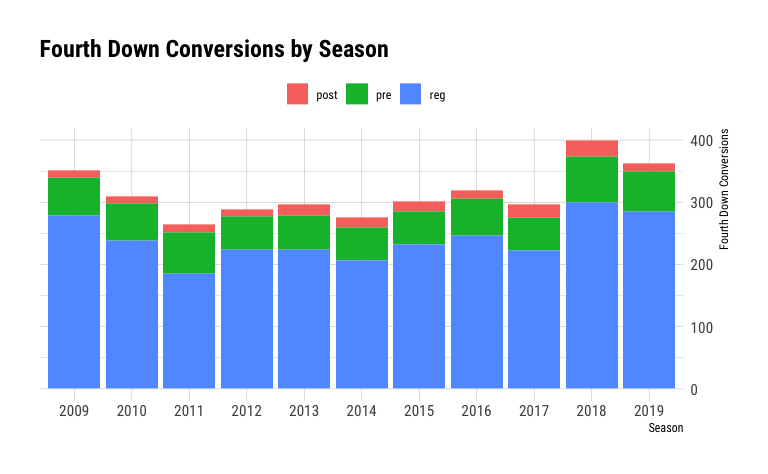
Plot Fourth Down Conversions by Season
ggplot(season_sum_fourth_downs, aes(x=season_nbr,
                                    y=fourth_down_conversions,
                                    fill=season_type_code)) +
  geom_col() +
  scale_y_continuous(position = "right") +
  scale_fill_discrete(name = "") +
  theme(legend.position="top") +
  ggtitle("Fourth Down Conversions by Season") +
  labs(x="Season", y="Fourth Down Conversions")
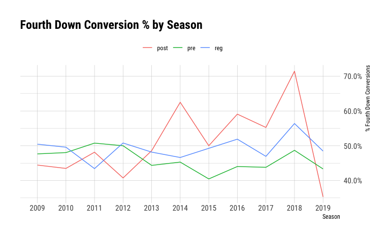
Plot % Fourth Down Conversions by Season
ggplot(season_sum_fourth_downs,
       aes(x=season_nbr,
           y=fourth_down_conversions/fourth_down_attempts,
           group=season_type_code,
           color=season_type_code
           )
       ) +
    geom_line() +
    scale_y_continuous(labels = scales::percent_format(), position = "right") +
    scale_color_discrete(name = "") +
    theme(legend.position="top") +
    ggtitle("Fourth Down Conversion % by Season") +
    labs(x="Season", y="% Fourth Down Conversions")
Summary
I hope this quick introduction to dbplyr gave you an idea of how to incorporate R and BigQuery into your data analysis flow. Being able to query BigQuery in a lazily executed fashion can help increase productivity by allowing us to combine database queries with in-memory manipulation in one operation, while also keeping down query cost.
Comments