
Multi-level Modeling in RStan and brms (and the Mysteries of Log-Odds)
Did you know you can now sign up for weekly-ish updates to our blog via email?
Overview
In this post we’ll take another look at logistic regression, and in particular multi-level (or hierarchical) logistic regression. We’ve seen Bayesian logistic regression before when we modeled field goals in NFL football earlier this year, and we used multi-level models before when we looked at Fourth-Down Attempts in NFL Football by team. This time we’ll try to build a bit more intuition around both. Also, this will be the first post I’ll tackle in R!
Why R?
R has been a mainstay in statistical modeling and data science for years, but more recently has been pinned into a needless competition with Python. In fact, R has a rich and robust package ecosystem, including some of the best statistical and graphing packages out there. R, along with Python and SQL, should be part of every data scientist’s toolkit. I’ve not used R in quite a while, in favor of Python and the occasional adventure in Julia, but it’s important to recognize that we should use the right tool for the job, not just always the one that’s most convenient. Especially using the tidyverse package ecosystem makes data wrangling (and increasingly modeling) code almost trivial and downright fun. I encourage folks that have been away from R for a bit to give it another go!
For this post, I’m using a few R libraries we’ll import first:
library(tidyverse)
library(broom.mixed)
library(janitor)
library(brms)
library(bayesplot)
library(hrbrthemes)
We’ll also want to use the handsome ipsum_rc theme from the hbrtheme package as our ggplot and bayesplot default:
theme_set(hrbrthemes::theme_ipsum_rc())
bayesplot_theme_set(hrbrthemes::theme_ipsum_rc())
Marketing Theme Park Season Passes
For this post, we’ll consider simulated sales data for a (hypothetical) theme park from chapter 9 of “R for Marketing Research and Analytics”, which inspired this post. This book really is a wide-ranging collection of statistical techniques to apply in various marketing settings and I often browse it for ideas, even if I don’t use the actual implementation.
Specifially, we’ll look at customer contacts representing attempts by the theme park to sell season passes via one of three channels - traditional mail, email and point-of-sale in the park - both as a standalone product and bundled with free parking.
The author’s have helpfully provided this data for us as a CSV with a permalink:
season_pass_data <- readr::read_csv("http://goo.gl/J8MH6A")
Let’s take a quick glimpse at the data. Looks like we have Bernoulli style data, with 3,156 records showing us whether the customer purchased a season pass (Pass), if they were presented with the bundle option (Promo) and through which Channel they were contacted:
glimpse(season_pass_data)
## Rows: 3,156
## Columns: 3
## $ Channel <chr> "Mail", "Mail", "Mail", "Mail", "Mail", "Mail", "Mail", "Mail…
## $ Promo   <chr> "Bundle", "Bundle", "Bundle", "Bundle", "Bundle", "Bundle", "…
## $ Pass    <chr> "YesPass", "YesPass", "YesPass", "YesPass", "YesPass", "YesPa…
All 3 columns are character columns, so we’ll want to convert them to useful factor and/or integer columns for modeling.
We’ll use dplyr to add a simple 1 count column n, and add factor columns for promo and channel. We’ll also convert the Pass variable to a Bernoulli style outcome variable of 0s and 1s.
season_pass_data <- season_pass_data %>%
    mutate(n = 1,
           bought_pass = case_when(Pass == "YesPass" ~ 1, TRUE ~ 0),
           promo = factor(Promo, levels = c("NoBundle", "Bundle")),
           channel = factor(Channel, levels = c("Mail", "Park", "Email"))
           )
When creating factor variables it’s usually a good idea to confirm the factor ordering to make sure it aligns with our expectations, which we can do with the contrasts function:
contrasts(season_pass_data$promo)
##          Bundle
## NoBundle      0
## Bundle        1
contrasts(season_pass_data$channel)
##       Park Email
## Mail     0     0
## Park     1     0
## Email    0     1
Next up, let’s convert our Bernoulli style data to Binomial data, by grouping and summarizing, to make our models run more efficiently.
season_pass_data_grp <- season_pass_data %>%
    group_by(promo, channel) %>%
    summarise(bought_pass = sum(bought_pass),
              n = sum(n)) %>%
    ungroup()

season_pass_data_grp
## # A tibble: 6 x 4
##   promo    channel bought_pass     n
##   <fct>    <fct>         <dbl> <dbl>
## 1 NoBundle Mail            359   637
## 2 NoBundle Park            284   333
## 3 NoBundle Email            27   512
## 4 Bundle   Mail            242   691
## 5 Bundle   Park            639   862
## 6 Bundle   Email            38   121
Exploring the Data
Next, let’s use dplyr and ggplot2 to look at a few different cuts of this data to get a sense of how we can answer some of the business questions we might encounter.
For example, we might get asked:
1) How many customers bought a season pass by channel, in a bundle or no bundle?
season_pass_data_grp %>%
    select(channel, promo, bought_pass) %>%
    pivot_wider(names_from = promo, values_from = bought_pass) %>%
    adorn_totals("col")
##  channel NoBundle Bundle Total
##     Mail      359    242   601
##     Park      284    639   923
##    Email       27     38    65
(Note: we use the extra-handy adorn_totals function from the janitor package here)
Or visually:
season_pass_data_grp %>%
    ggplot(aes(x = channel, y = bought_pass, group = promo, fill = promo)) +
    geom_col() +
    scale_y_continuous() +
    scale_fill_ft() +
    labs(x = "",
       y = "# Bought Season Pass",
       title = "Customers by Channel",
       subtitle = "by Promotion (Bundle/NoBundle)"
       )
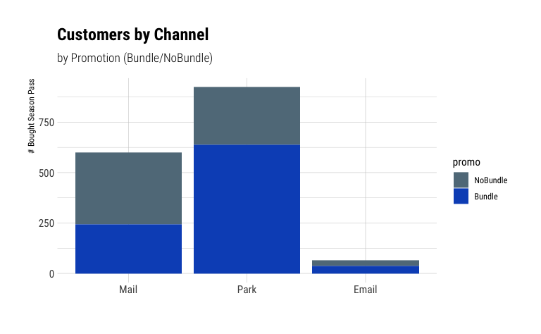
We note that Park is our biggest sales channel, while Email had by far the lowest overall sales volume.
2) What percentage of customers bought a season pass by channel, in a bundle or no bundle?
season_pass_data_grp %>%
    group_by(channel) %>%
    summarise(bought_pass = sum(bought_pass),
              n = sum(n),
              percent_bought = bought_pass/n) %>%
    ggplot(aes(x = channel,
               y = percent_bought,
               fill = channel,
               label = scales::percent(percent_bought))) +
    geom_col(width = .5) +
    coord_flip() +
    theme(legend.position = "none") +
    geom_text(hjust = "outward", nudge_y=.01, color="Black") +
    scale_fill_ft() +
    scale_y_continuous(labels = NULL) +
    labs(x = "",
       y = "% Bought Season Pass by Channel",
       title = "% of Customers by Channel"
       )
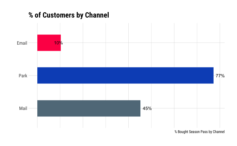
Email seems to also have the lowest take rate of all channels, with only 10% of contacted customer buying a season pass. At the same time, the high take rate (77%) of customers in the park could be indication of selection basis, wherein customers already in the park have demonstrated a higher propensity to purchase theme park passes.
3) What percentage of customers that bought a season pass bought it in a bundle by channel?
season_pass_data_grp %>%
    select(channel, promo, bought_pass) %>%
    pivot_wider(names_from = promo, values_from = bought_pass) %>%
    mutate(percent_bundle = Bundle/(NoBundle + Bundle)) -> season_pass_data_grp_pct_bundle

season_pass_data_grp_pct_bundle
## # A tibble: 3 x 4
##   channel NoBundle Bundle percent_bundle
##   <fct>      <dbl>  <dbl>          <dbl>
## 1 Mail         359    242          0.403
## 2 Park         284    639          0.692
## 3 Email         27     38          0.585
season_pass_data_grp_pct_bundle %>%
    ggplot(aes(x = channel,
               y = percent_bundle,
               fill = channel,
               label = scales::percent(percent_bundle)
               )
           ) +
    geom_col(width = .5) +
    coord_flip() +
    theme(legend.position = "none") +
    geom_text(hjust = "outward", nudge_y=.01, color="Black") +
    scale_y_continuous(labels = NULL) +
    scale_fill_ft() +
    labs(x = "",
       y = "% Bought Season Pass w/Bundle",
       title = "% of Bundle Customers by Channel"
       )
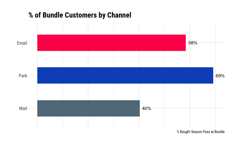
Again, customers in the park have the highest percentage of season passes sold in the bundle. We could argue that since they’re already showing higher motivation to buy a season pass, the upsell to a pass bundled with parking is comparatively easier.
Interestingly, almost 60% of customers contacted via email that purchased a season pass bought it as part of the bundle.
Given the relatively small number of overall email-attributed sales, it makes sense to investigate further here to see if bundling is in fact a valuable sales strategy for digital channels vs mail and in the park.
A Baseline Model
In classical modeling, our first instinct here would be to model this as logistic regression, with bought_pass as our response variable. So, if we wanted to measure the overall effectiveness of our bundle offer, we’d set up a simple model using the glm module and get a summary of estimated coefficients. However, as good Bayesians that value interpretable uncertainty intervals, we’ll go ahead and use the excellent brms library that makes sampling via RStan quite easy.
We’ll set reasonably high value for the number of sampler iterations and set a seed for more repeatable sampling results:
# iterations to use for MCMC sampling
iter <- 10000
set.seed(42)
Instead of relying on the default priors in brms, we’ll use a (Normal(0, 1)) prior for intercept and slope.
Let’s do a quick check to see what that looks like:
draws <- 1000
norm_df <- as_tibble(data.frame(sd_1 = rnorm(draws, mean = 0, sd = 1),
                      sd_2 = rnorm(draws, mean = 0, sd = 2),
                      sd_5 = rnorm(draws, mean = 0, sd = 5))) %>%
    pivot_longer(cols = c(sd_1, sd_2, sd_5), names_to = "prior", values_to = "samples")

ggplot(norm_df, aes(y = fct_rev(prior), x=samples, fill = stat(abs(x) < 2.5))) +
    stat_halfeye() +
    scale_fill_manual(values = c("gray80", "skyblue")) +
    labs(title = "Normal distribution priors",
         x = "log-odds",
         y  = "stdev")
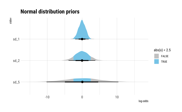
This shows us that our (Normal(0, 1)) prior reasonably supports effect sizes from ~-2.5 to ~2.5 in log-odds terms, while a sd of 5 would likely be too diffuse for a marketing application.
base_line_promo_model <- brm(bought_pass | trials(n) ~ 1 + promo,
                             prior = c(prior(normal(0, 1), class = Intercept),
                                       prior(normal(0, 1), class = b)),
                             data = season_pass_data_grp,
                             family = binomial(link = "logit"),
                             iter = iter,
                             cores = 4,
                             backend="cmdstan",
                             refresh = 0
                             )
We’ll take a quick look at chain divergence, mostly to introduce the excellent mcmc plotting functions from the bayesplot package.
mcmc_trace(base_line_promo_model, regex_pars = c("b_"), facet_args = list(nrow = 2))
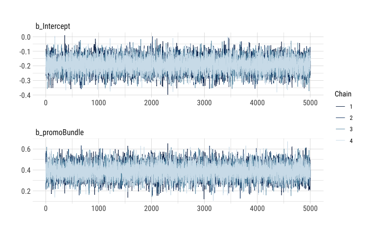
We note that our chains show convergence and are well-mixed, so we move on to taking a look at the estimates:
summary(base_line_promo_model, prob = 0.89)
##  Family: binomial
##   Links: mu = logit
## Formula: bought_pass | trials(n) ~ 1 + promo
##    Data: season_pass_data_grp (Number of observations: 6)
## Samples: 4 chains, each with iter = 10000; warmup = 5000; thin = 1;
##          total post-warmup samples = 20000
##
## Population-Level Effects:
##             Estimate Est.Error l-89% CI u-89% CI Rhat Bulk_ESS Tail_ESS
## Intercept      -0.19      0.05    -0.27    -0.11 1.00    14729    13089
## promoBundle     0.39      0.07     0.28     0.50 1.00    16323    13076
##
## Samples were drawn using sample(hmc). For each parameter, Bulk_ESS
## and Tail_ESS are effective sample size measures, and Rhat is the potential
## scale reduction factor on split chains (at convergence, Rhat = 1).
mcmc_areas(
    base_line_promo_model,
    regex_pars = "b_",
    prob = 0.89,
    point_est = "median",
    area_method = "equal height"
    ) +
    geom_vline(xintercept = 0, color = "red", alpha = 0.6, lwd = .8, linetype = "dashed") +
    labs(
        title = "Effect of Bundle Promotion on Sales"
    )
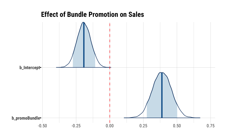
The slope coefficient promoBundle is positive and does not contain 0 in the uncertainty interval. The value of 0.39 represents the effect of the Bundle treatment in terms of log-odds, i.e. bundling increases the log odds of buying a season pass by 0.39. We can convert that to a % by exponentiating the coefficients (which we get via fixef) to get the % increase of the odds:
exp(fixef(base_line_promo_model))
##              Estimate Est.Error      Q2.5     Q97.5
## Intercept   0.8252316  1.053328 0.7460204 0.9136109
## promoBundle 1.4739224  1.073539 1.2850493 1.6936006
In terms of percent change, we can say that the odds of a customer buying a season pass when offered the bundle are 47% higher than if they’re not offered the bundle.
Aside: what the heck are log-odds anyway?
Log-odds, as the name implies are the logged odds of an outcome. For example, an outcome with odds of 4:1, i.e. a probability of 80% (4/(4+1)) has log-odds of log(4/1) = 1.386294.
Probability, at its core is just counting. Taking a look at simple crosstab of our observed data, let’s see if we can map those log-odds coefficients back to observed counts.
season_pass_data %>%
    group_by(promo) %>%
    summarise(bought_pass = sum(bought_pass),
              did_not_buy = sum(n) - sum(bought_pass)) %>%
    adorn_totals(c("row", "col"), name="total") %>%
    mutate(percent_bought = bought_pass/total)
##     promo bought_pass did_not_buy total percent_bought
##  NoBundle         670         812  1482      0.4520918
##    Bundle         919         755  1674      0.5489845
##     total        1589        1567  3156      0.5034854
We estimated an intercept of -0.19, which are the log-odds for NoBundle (the baseline). We observed 670 of 1,482 customers that were not offered the bundle bought a season pass vs 812 that didn’t buy. With odds defined as bought/didn’t buy, the log of the NoBundle buy odds is:
odds_no_bundle <- 670/812
log(odds_no_bundle)
## [1] -0.1922226
While our estimated slope of 0.39 for Bundle is the log of the ratio of buy/didn’t buy odds for Bundle vs NoBundle:
odds_no_bundle <- 670/812
odds_bundle <- 919/755
log(odds_bundle/odds_no_bundle)
## [1] 0.388791
If we do this without taking any logs,
odds_no_bundle
## [1] 0.8251232
odds_bundle/odds_no_bundle
## [1] 1.475196
we see how this maps back to the exponentiated slope coefficient from the model above:
exp(fixef(base_line_promo_model))
##              Estimate Est.Error      Q2.5     Q97.5
## Intercept   0.8252316  1.053328 0.7460204 0.9136109
## promoBundle 1.4739224  1.073539 1.2850493 1.6936006
We can think of 1.47 as the odds ratio of Bundle vs NoBundle, where ratio of 1 would indicate no improvement.
What’s more, we can link the overall observed % of sales by Bundle vs Bundle to the combination of the coefficients. For predictive purposes, logistic regression in this example would compute the log-odds for a case of NoBundle (0) roughly as:
plogis(-0.19 + 0.39*0)
## [1] 0.4526424
And Bundle (1) as :
plogis(-0.19 + 0.39*1)
## [1] 0.549834
Which maps back to our observed proportions of 45% and 55% in our counts above.
We can also show this via the predict function for either case:
newdata <- data.frame(promo = factor(c("NoBundle", "Bundle")), n = 1)

predict(base_line_promo_model, newdata)[c(1:2)]
## [1] 0.4585 0.5473
Logistic regression is probably one of the most underrated topics in modern data science.
(Thanks to the folks at he UCLA Stats department for this detailed writeup on this topic.)
Is this the right model?
Back to our model!
However, this simple model fails to take Channel into consideration and is not actionable from a practical marketing standpoint where channel mix is an ever-present optimization challenge. In other words, while the model itself is fine and appears to be a good fit, it’s not really an appropriate “small world” model for our “large world”, to invoke Richard McElreath.
Simply modeling Channel as another independent (dummy) variable would also likely misrepresent the actual data generating process, since we know from our EDA above that Channel and Promo seem to depend on one another.
So, let’s try to model this dependency with another common technique in classical modeling, interaction terms.
Modeling Interactions
Again using the brms library, it’s easy to add interaction terms using the * formula convention familiar from lm and glm. This will create both individual slopes for each variable, as well as the interaction term:
promo_channel_model_interactions <- brm(bought_pass | trials(n) ~ promo*channel,
                                        prior = c(prior(normal(0, 1), class = Intercept),
                                                  prior(normal(0, 1), class = b)),
                                        data = season_pass_data_grp,
                                        family = binomial(link = "logit"),
                                        iter = iter,
                                        backend="cmdstan",
                                        cores = 4,
                                        refresh = 0)
Again, our model converged well and we observe well-mixed chains in the traceplot:
mcmc_trace(promo_channel_model_interactions, regex_pars = c("b_"), facet_args = list(nrow = 3))
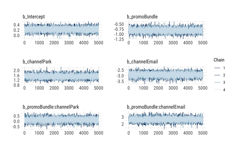
(We’ll forgo convergence checks from here on out for this post, but it’s never a bad idea to inspect your chains for proper mixing and convergence.)
summary(promo_channel_model_interactions, prob = 0.89)
##  Family: binomial
##   Links: mu = logit
## Formula: bought_pass | trials(n) ~ promo * channel
##    Data: season_pass_data_grp (Number of observations: 6)
## Samples: 4 chains, each with iter = 10000; warmup = 5000; thin = 1;
##          total post-warmup samples = 20000
##
## Population-Level Effects:
##                          Estimate Est.Error l-89% CI u-89% CI Rhat Bulk_ESS
## Intercept                    0.22      0.08     0.10     0.35 1.00    16399
## promoBundle                 -0.82      0.11    -1.00    -0.64 1.00    13436
## channelPark                  1.51      0.17     1.24     1.78 1.00    12793
## channelEmail                -2.93      0.19    -3.24    -2.63 1.00    13227
## promoBundle:channelPark      0.14      0.20    -0.18     0.46 1.00    11813
## promoBundle:channelEmail     2.63      0.28     2.19     3.08 1.00    13049
##                          Tail_ESS
## Intercept                   15553
## promoBundle                 13047
## channelPark                 12602
## channelEmail                12513
## promoBundle:channelPark     11875
## promoBundle:channelEmail    12768
##
## Samples were drawn using sample(hmc). For each parameter, Bulk_ESS
## and Tail_ESS are effective sample size measures, and Rhat is the potential
## scale reduction factor on split chains (at convergence, Rhat = 1).
mcmc_areas(
    promo_channel_model_interactions,
    regex_pars = "b_",
    prob = 0.89,
    prob_outer = 1,
    point_est = "median",
    area_method = "equal height"
    ) +
    geom_vline(xintercept = 0, color = "red", alpha = 0.6, lwd = .8, linetype = "dashed") +
    labs(
        title = "Effect of Channel and Bundle Promotion",
        subtitle = "with interactions"
    )
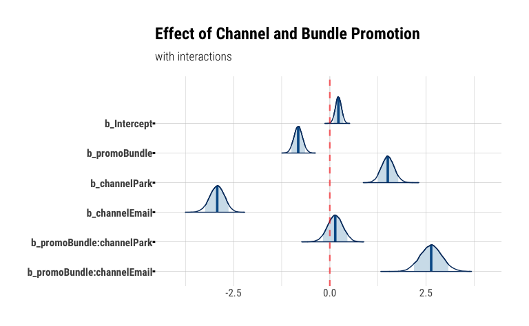
Three things immediately come to our attention:
- the
Emailchannel is associated with a -2.93 decrease in log odds of selling a season pass (vs the baseline channelMail) - however, the interaction term
promoBundle:channelEmail, i.e. the effect of theBundlepromo given theEmailchannel shows a ~2.6x increase in log-odds over the baseline - interestingly, the
Parkchannel does not seem to meaningfully benefit from offering a bundle promotion, shown by the fact that its posterior uncertainty interval spans0
So, while Email itself has shown to be the least effective sales channel, we see that offering a bundle promotion in emails seems to make the most sense. Perhaps, customers on our email list are more discount motivated than customers in other channels.
At the same time, our customers in the park, as we’ve speculated earlier, seem to have higher price elasticity than mail or email customers, making the park a better point-of-sale for non-bundled (and presumably non-discounted) SKUs.
In “R for Marketing Research and Analytics”, the authors also point out that the interaction between channel and promo in this data points to a case of Simpson’s Paradox where the aggregate effect of promo is different (potentially and misleading), compared to the effect at the channel level.
Multi-Level Modeling
Interaction terms, however useful, do not fully take advantage of the power of Bayesian modeling. We know from our EDA that email represent a small fraction of our sales. So, when computing the effects of Email and Promo on Email, we don’t fully account for inherent lack of certainty as a result of the difference in sample sizes between channels. A more robust way to model interactios of variables in Bayesian model are multilevel models. They offer both the ability to model interactions (and deal with the dreaded collinearity of model parameters) and a built-in way to regularize our coefficient to minimize the impact of outliers and, thus, prevent overfitting.
In our case, it would make the most sense to model this with both varying intercepts and slopes, since we observed that the different channels appear to have overall lower baselines (arguing for varying intercepts) and also show different effects of offering the bundle promotion (arguing for varying slopes). In other cases though, we may need to experiment with different combinations of fixed and varying parameters.
Luckily, it’s a fairly low-code effort to add grouping levels to our model. We will model both a varying intercept (1) and varying slope (promo) by channel, removing the standard population level intercept (0) and slope.
promo_channel_model_multilevel <- brm(bought_pass | trials(n) ~ 0 + (1 + promo | channel),
                                        prior = c(
                                            prior(normal(0, 1), class = sd)
                                            ),
                                        data = season_pass_data_grp,
                                        control = list(adapt_delta = 0.95),
                                        family = binomial(link = "logit"),
                                        iter = iter,
                                        cores = 4,
                                        backend="cmdstan",
                                        refresh = 0
                                        )
This time we’ll use the broom package to tidy up the outputs of our model so that we can inspect the varying parameters of our model more easily:
tidy(promo_channel_model_multilevel, prob = 0.89, effects = c("ran_vals")) %>% filter(group == "channel")
## # A tibble: 6 x 9
##   effect   component group  level term     estimate std.error conf.low conf.high
##   <chr>    <chr>     <chr>  <chr> <chr>       <dbl>     <dbl>    <dbl>     <dbl>
## 1 ran_vals cond      chann… Mail  (Interc…    0.250    0.0800   0.0937     0.408
## 2 ran_vals cond      chann… Park  (Interc…    1.75     0.155    1.45       2.06
## 3 ran_vals cond      chann… Email (Interc…   -2.82     0.193   -3.22      -2.46
## 4 ran_vals cond      chann… Mail  promoBu…   -0.859    0.113   -1.08      -0.638
## 5 ran_vals cond      chann… Park  promoBu…   -0.695    0.172   -1.04      -0.362
## 6 ran_vals cond      chann… Email promoBu…    1.98     0.276    1.44       2.53
Another benefit of multi-level models is that each level is explicitly modeled, unlike traditional models where we typically model n-1 coefficients and are always left to interpret coefficients against some un-modeled baseline.
From the output above, we can see that Email in general is still performing worse vs the other channels judging from its low negative intercept, while the effect of the Bundle promo for the Email channel is positive at ~2 increase in log-odds. However, compared to our single-level interaction models, we see that the multilevel model did a better job constraining the estimate of the effect of offering the bundle in emails by shrinking the estimate a bit towards the group mean.
Visualizing this as a ridge plot, it’s more clear how the Bundle effect for Email is less certain than for other models, which makes intuitive sense since we have a lot fewer example of email sales to draw on. However, it appears to be the only channel where bundling free parking makes a real difference in season pass sales.
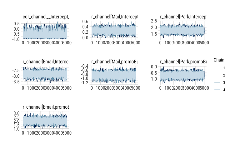
mcmc_areas(
    promo_channel_model_multilevel,
    regex_pars = "r_channel",
    prob = 0.89,
    point_est = "median",
    area_method = "equal height"
    ) +
    geom_vline(xintercept = 0, color = "red", alpha = 0.6, lwd = .8, linetype = "dashed") +
    labs(
        title = "Effect of Channel and Bundle Promotion",
        subtitle = "multi-level model: varying intercept and slope"
    )
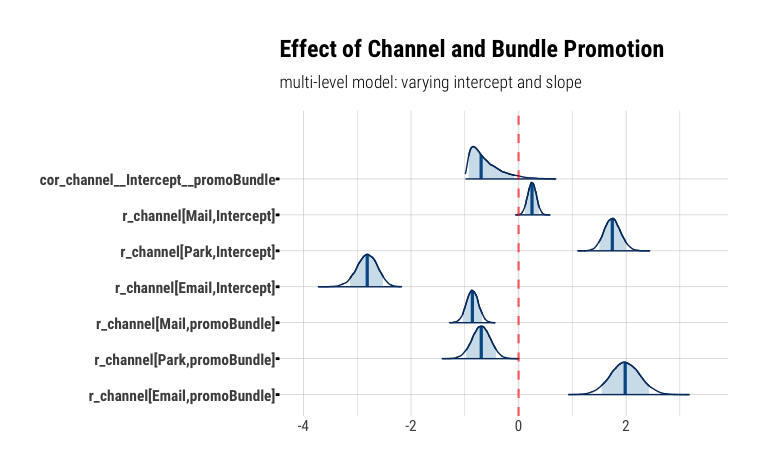
So, while we’ve seen that email response and take rates are the lowest of all channels, we can confidently tell our marketing partners that offering bundling via email has a positive effect that is worth studying more and gathering more data. Since email tends to be a cheaper alternative to conventional in-home mails, and certainly cheaper than shuttling people into the park, the lower response rate needs to be weighed against channel cost.
Model Comparison
It’s worth noting that both the model with interactions and the multilevel model predict essentially about the same probabilities for bundled sales via email or in the park. We can see from our plots that while the interactions model has more extreme estimates for intercept and interaction term, the multilevel model constrains both the intercept for each channel and the varying slopes for each channel towards the group mean. So, while in the multilevel model we estimate a lower slope for email (1.99 vs 2.63), we also estimate a slightly higher intercept for email (-2.82 vs -2.93), resulting in roughly the same prediction as the interaction model.
newdata_channel <- data.frame(promo = factor(c("Bundle", "Bundle")),
                              channel = factor(c("Email", "Park")), n = 1)

predict(promo_channel_model_interactions, newdata_channel)
##      Estimate Est.Error Q2.5 Q97.5
## [1,]  0.29150 0.4544646    0     1
## [2,]  0.74305 0.4369625    0     1
predict(promo_channel_model_multilevel, newdata_channel)
##      Estimate Est.Error Q2.5 Q97.5
## [1,]  0.30065 0.4585522    0     1
## [2,]  0.73850 0.4394626    0     1
The advantage for the multilevel model in this case really comes from the ability to regularize the model more efficiently, and to be able to more easily interpret the coefficients. In more complex modeling challenges, multilevel models really shine when there are more than one and/or nested grouping levels (hence “multilevel”).
Summary
Let’s wrap up with a few take aways:
- Although it might have been obvious in this example dataset, but a first step in modeling is to make sure our model captures the true data generating process adequately, so we can ultimately answer the most meaningful business questions with confidence. So, even a well fitting model may be the wrong model in a given context. Or in short, make sure “small world” represents “large world” appropriately.
- Interaction terms are an easy first step to add dependencies to our model. However, for larger models with many coefficients, they can become difficult to interpret and don’t easily allow for regularization of parameters.
- From a modeling perspective, multi-level models are a very flexible way to approach regression models. They allow us to encode relationships that help create stronger estimates by pooling (sharing) data across grouping levels, while also helping to regularize estimates to avoid overfitting.
- Through libraries like
brms, implementing multilevel models in R becomes only somewhat more involved than classical regression models coded inlmorglm.
So, for anything but the most trivial examples, Bayesian multilevel models should really be our default choice.
Resources
You can find the R Markdown file for this post here: https://github.com/clausherther/rstan/blob/master/hierarchical_modelng_r_stan_brms_season_pass.Rmd
I’ve found these links helpful whenever I’ve worked on multi-level Bayesian models and/or R:
- Richard McElreath’s book, Statistical Rethinking, including his invaluable lectures on video
- Solomon Kurz’ adaptation of Statisticial Rethinking to the tidyverse
- The R Graph Gallery
- HBR Themes for ggplot
- The
brmspackage documentation - The Stan User Guide
- “FAQ: HOW DO I INTERPRET ODDS RATIOS IN LOGISTIC REGRESSION?”
- “R for Marketing Research and Analytics”
Comments